This article requires having read the first article on Speaker Verification using GMM-UBM method to fully understand what this approach brings.
In the paper Support Vector Machines using GMM Supervectors for Speaker Verification by W. M. Campbell, D. E. Sturim, D. A. Reynolds, authors introduce a new approach, different from the MAP adaptation of means on the GMM models for speaker verification tasks.
GMM super-vectors
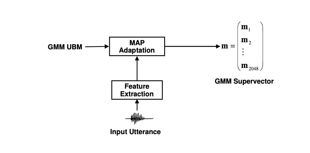
SVM-based method, as GMM-UBM method, rely on GMM vectors, but in a stacked format, called GMM super-vectors.
During the enrollment, we extract the means of the GMMs after adaptation with MAP from the UBM, but instead of using those to score the new test samples, the authors introduce this notion of super-vector as simply the stacked means of the mixture components. These vector is then fed as an input to a Support Vector Machine Classifier (SVM) with 2 classes.

For example, instead of having 512 Gaussian components of dimention 26 each, we have a single vector of size \(512 \times 26 = 13312\).
SVM classification
Support Vector Machine (SVM) algorithm learns a discriminative frontier between two classes which maximizes margins. It can leverage a non-linear kernel mapping to project the data in a high-dimensional space in which it is linearly separable.
The two classes to distinguish from are simply:
- the target speaker
- the impostor/background/population
The discriminative function of the SVM is given by:
\[f(x) = \sum_{i=1}^N \alpha_i y_i K(x, x_i) + d\]Where:
- \(y_i\) is the ground truth for the output value, either 1 or -1.
- \(x_i\) is the support vector
- \(\alpha_i\) are the corresponding weights
- \(d\) is a bias term
The SVM can be linearly separable if we apply a kernel function \(K(x,y) = b(x)^t b(y)\), where \(b(x)\) is a mapping function from the input space to a possibly infinite dimensional space. This method is called the Kernel trick.
And that’s it ! We just need to train the SVM model on GMM super-vectors with positive and negative labels. Applying a SVM with a non-linear Kernel will identify the discriminative frontier.
The prediction is straight-forward, since we just need to extract the super-vector and run it into the trained SVM.
