
The method introduced below is called GMM-UBM, which stands for Gaussian Mixture Model - Universal Background Model. This method has, for a long time, been a state-of-the-art approach.
I will use as a reference the paper: “A Tutorial on Text-Independent Speaker Verification” by Frédétic Bimbot et al. Although from 2002, this tutorial describes this classical approach pretty well.
This article requires that you have understood the basics of Speaker Verification.
In this article, I will present the main steps of a Speaker Verification system.
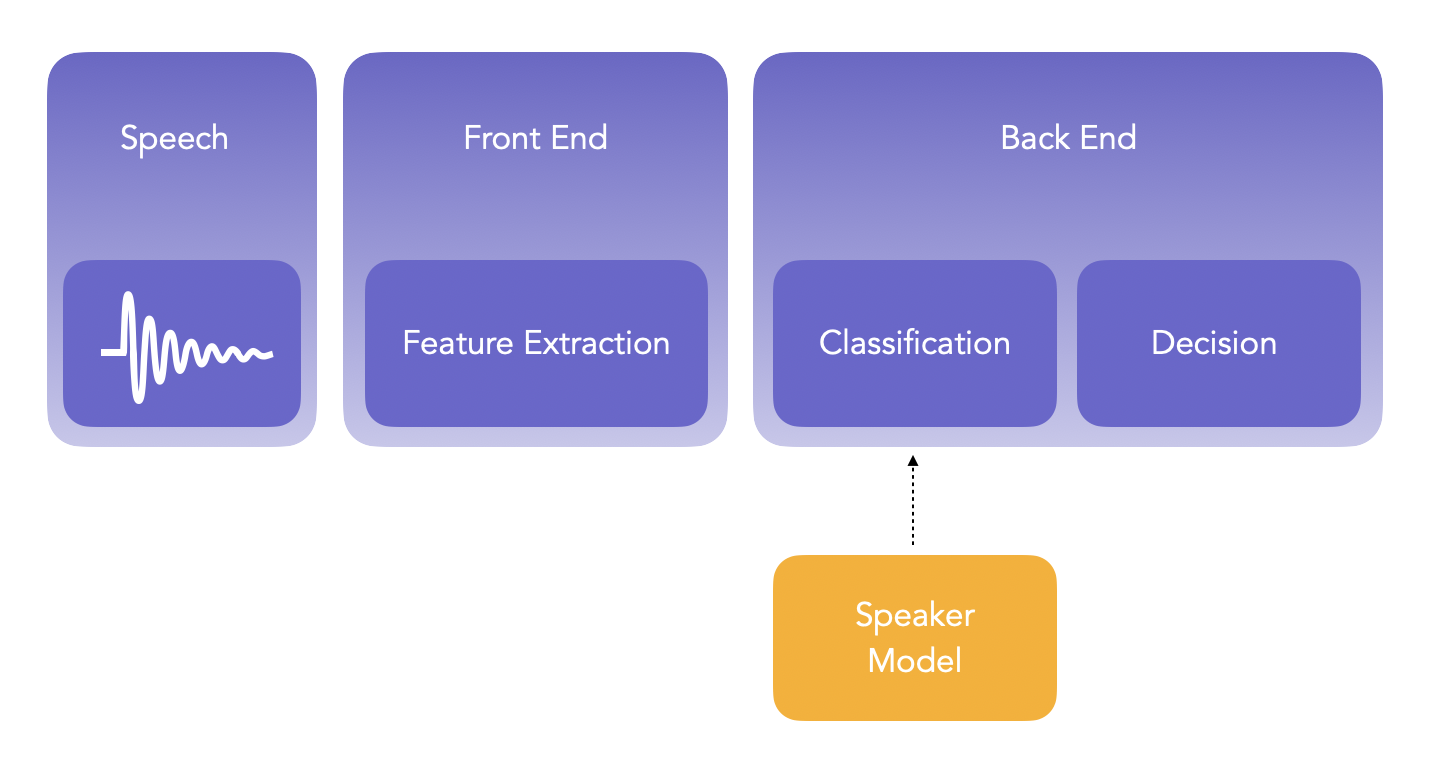
The main steps of speaker verification are:
- Development: learn speaker-idenpendent models using large amount of data. This is a pre-training part, called a Universal Background Model (UBM). It can be gender-specific, in the sense that we have 1 for Males, and 1 for Females.
- Enrollment: learn distinct characteristics of a speaker’s voice. This step typically creates one model per unique speaker considered. This is the training part.
- Verification: distinct characteristics of a claimant’s voice are compared with previously enrolled claimed speaker models. This is the prediction part.
The first step is to extract features from the development set, enrollment set and verification set.
I. Speech acquisition and Feature extraction
We should extract features from the signal to convert the raw signal into a sequence of acoustic feature vectures which we will use to identify the speaker. We make the assumption that each audio sample that we have contains only one speaker.
Most speech features used in speaker verification rely on a cepstral representation of speech.
1. Filterbank-based cepstral parameters (MFCC)
Pre-emphasis
The first step is usually to apply a pre-emphasis of the signal to enhance the high frequencies of the spectrum, reduced by the speech production process:
\[x_p(t) = x(t) - a x(t-1)\]Where \(a\) takes values between 0.95 and 0.98.
Framing
The signal is then split into successive frames. Most of the time, a length of frame of 20 milliseconds is used, with a shift of 10 milliseconds.
Windowing
Then, a windowing is applied. Indeed, when you cut your signal into frames, it is most likely that the end of a frame will not match the start of the next frame. Therefore, a windowing function is needed. The Hamming window is one of the most common approaches. Windowing also gives a more accurate idea of the original signal’s frequency spectrum, as is “cuts off” signals at their end.
The Hamming window is given by:
\[w[n]=a_{0}-\underbrace {(1-a_{0})} _{a_{1}}\cdot \cos \left({\tfrac {2\pi n}{N}}\right),\quad 0\leq n\leq N\]Where \(a_0 = 0.53836\) is the optimal value.
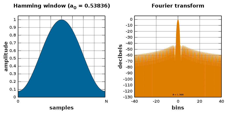
All windowing functions can be found on Wikipedia.
Fast Fourier Transform (FFT)
Then, a FFT algorithm is picked (most often Cooley–Tukey) to compute efficiently the Discrete Fourrier Transform (DFT):
\[X_{k}=\sum _{n=0}^{N-1}x_{n}e^{-i2\pi kn/N}\qquad k=0,\ldots ,N-1\]We typically make the computation on 512 points.
Modulus
The absolute value of the FFT is then computed, which gives the magnitude. At that point, we have a power spectrum sampled over 512 points. However, since the spectrum is symmetric, only half of those points are useful.
Mel Filters
The spectrum at that point has lots of fluctuations, and we don’t need them. We need to apply a smoothing, which will reduce the size of the spectral vectors. We therefore multiply the spectrum by a filterbank, a series of bandpass frequency filters.
Filters can be central, right or left, and defined by their shape (triangular most often). A common choice is the Bark/Mel scale for the frequency localization, a scale similar to the frequency scale of the human ear. A Mel is a unit of measure based on the human ears perceived frequency. It does not correspond linearly to the physical frequency of the tone, as the human auditory system apparently does not perceive pitch linearly. The Mel scale is approximately a linear frequency spacing below 1 kHz and a logarithmic spacing above 1 kHz. See more here.
\[f_{MEL} = 2595 * \log_{10} ( {1 + \frac{f}{700}} )\]Where \(f\) is the physical frequency in Hz, and \(f_{MEL}\) should be close to the percieved frequency.
We can now compute the Mel spectrum of the magnitude spectrum:
\[s(m) = \sum_{k=0}^{N-1} [ {\mid X(k) \mid}^2 H_m(k) ]\]Where \(H_m(k)\) is the weight given to the \(k^{th}\) energy spectrum bin contributing to the \(m^{th}\) output band.
Discrete Cosine Transform (DCT)
Finally, we take the log of the spectrum and a Discrete Cosine Transform is applied. We obtain the Mel-Frequency Cepstral Coefficients (MFCC), and since most of the information is gathered in the first few coefficients, we can only select the first few ones (usually 12 or 20).
\[c_n = \sum_{m=0}^{M-1} log_{10}(s(m)) cos(\frac{\pi}{M} n(m-\frac{1}{2}))\]There we are, we obtained the MFCC coefficients describing the input signal window.
Cepstral Mean Substraction (CMS)
Finally, and espacially in Speaker Verification tasks, the cepstral mean vector is substracted from each vector. This step is called Cepstral Mean Substraction (CMS) and removes slowly varying convolutive noises.
Cepstral mean variance normalization (CMVN)
Cepstral mean variance normalization (CMVN) minimizes distortion by noise contamination for robust feature extraction by linearly transforming the cepstral coefficients to have the same segmental statistics (mean 0, variance 1).
It is however known to degrade the performance of speaker verification tasks on short utterances.
2. LPC-based cepstral parameters
In Linear Predictive Coding (LPC) analysis, we represent the audio using the information of linear predictive models. We first split the input signal into the fundamental elements of the speech production apparatus:
- the glottal source, (the space between the vocal folds) produces the buzz, characterizes the intensity (loudness) and frequency (pitch)
- the vocal tract (the throat and mouth) forms the tube, which is characterized by its resonances
- the nasal tract
- the lips, generates hisses and pops
And we model each of the with an Auto Regressive filter on each window. More specifically:
- a lowpass filter for the glottal source
- an AR filter for the vocal tract
- an ARMA filter for the nasal tract
- an MA filter for the lips
Overall, the speech production process becomes an ARMA process, simplified in an AR process. We take each window and estimate the coefficients of an AR filter on the speech signal.
\[c_0 = ln(\sigma^2)\] \[c_m = a_m + \sum_{k=1}^{m-1} (\frac{k}{m}) c_k a_{m-k}, 1 ≤ m ≤ p\] \[c_m = \sum_{k=1}^{m-1} (\frac{k}{m}) c_k a_{m-k}, p < m\]Where \(\sigma^2\) is the gain term in LPC model, \(a_m\) are the LPC coefficients and \(p\) the number of LPC coefficients calculated.
There are many other features to extract, but MFCCs are the most frequent ones, LPC is sometimes used, so I won’t dive deeper in this.
3. Voice Activity Detection
We might now want to discard useless information in the frames we extracted features for. We do so by removing frames that do not contain speech using Voice Activity Detection (VAD).
A common approach is the Gaussian-based VAD, but one can also use the energy-based VAD. The aim of a VAD is to aquire speech only when it occurs. I described a bit further the concept and implementation of Voice Activity Detection in this project.
The main steps behind building a VAD are:
- Break audio signal into frames
- Extract features from each frame
- Train a classifier on a known set of speech and silence frames (could ba a gaussian model or a rule-based decision)
- Classify unseen frames as speech or silence
VAD performs well on audio with relatively low signal-to-noice ratio (SNR), a ratio which compares the level of a desired signal to the level of background noise.
II. Statistical Modeling
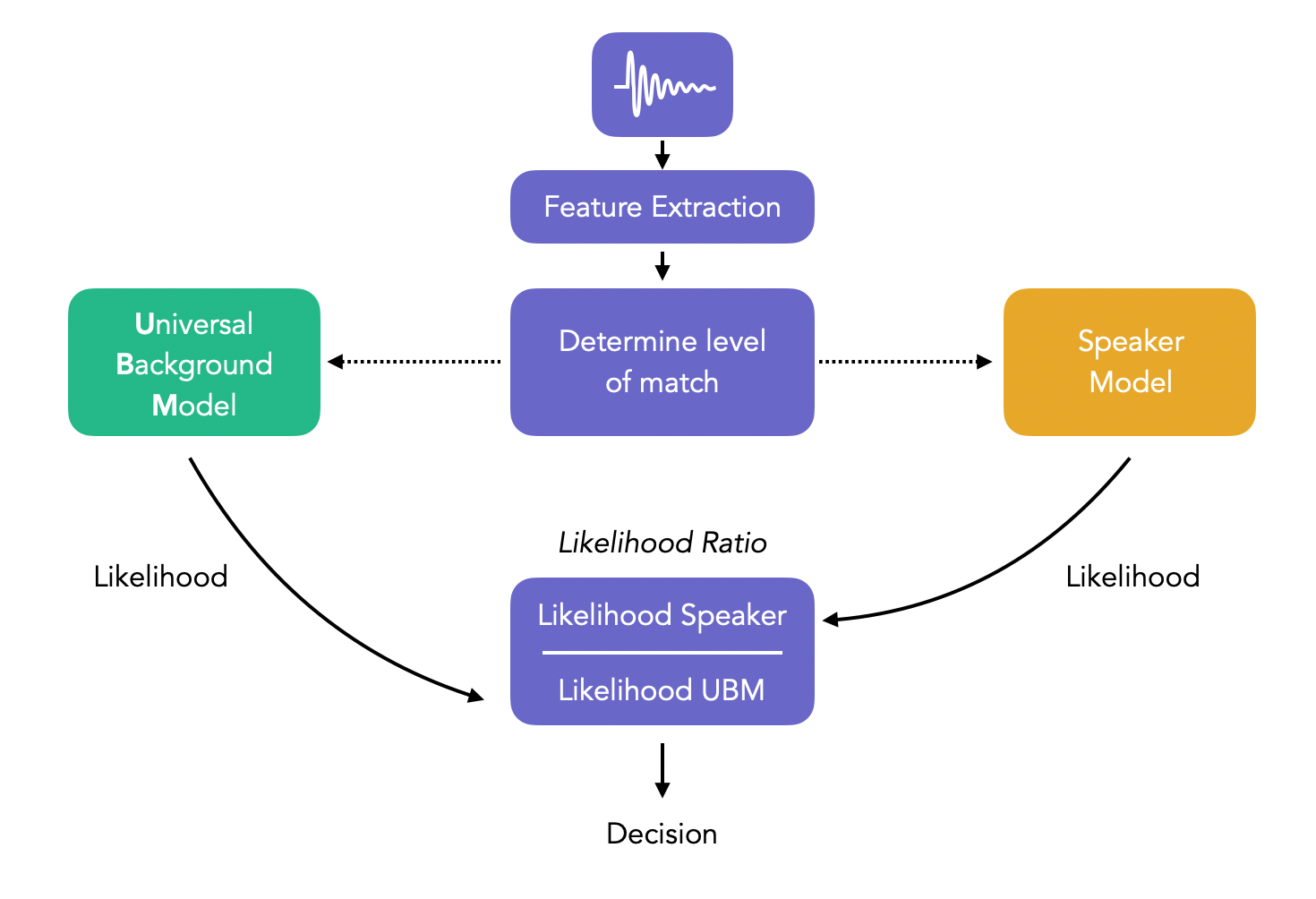
The core of the speaker verification decision is the likelihood ratio. Say that we want to determine if speech sample Y (from the verification set) was spoken by S.
Then, the verification task is a basic hypothesis testing:
\(H_0\) : Y is from speaker S \(H_1\) : Y is not from speaker S
The test to decide whether to accept \(H_0\) or not is the Likelihood Ratio (LR):
\[LR = \frac{p(Y \mid H_0)}{p(Y \mid H_1)}\]If the Likelihood ratio is greater than the threshold \(\theta\), we accept \(H_0\), otherwise we accept \(H_1\).
If we talk in terms of logs, then the log-likelihood ration is simply the difference between the logs of the 2 probability density functions:
\[\log(LR) = \log(p(Y \mid H_0)) - \log(p(Y \mid H_1))\]We have a speaker to test for \(H_0\), and we can build a model, say \(\lambda_{hyp}\), being for example a Gaussian Distribution of the features extracted.
However, we do not have an alternative model for \(H_1\). We must compute what is called a “Background Model”, which would be a Gaussian Model \(\lambda_{\overline{hyp}}\).
There are 2 options for the background model:
- either consider the closed set of other speakers and compute: \(p(X \mid \lambda_{\overline{hyp}}) = f ( p(X \mid \lambda_1), ..., p(X \mid \lambda_N))\), where \(f\) is an aggregative function like the mean or the max. It however requires a model per alternative hypothesis, i.e. per speaker
- or consider a pool of several different speakers to train a single model, called the Universal Background Model (UBM)
The main advantage of the UBM is that it is universal in the sense that it can be used by any of the speakers, without having to re-train a model.
The pipeline can be represented as such:
1. Universal Background Model : Development
A UBM is a high-order Gaussian Mixture Model (usually 512 to 2048 mixtures with 24 dimensionsa) trained on a large quantity of speech, from a wide population. This step is used to learn speaker-independent distribution of features, used in the alternative hypothesis in the likelihood ratio.
For a D-dimensional feature vector \(x\), the mixture density is:
\[P(x \mid \lambda) = \sum_{k=1}^M w_k \times g(x \mid \mu_k, \Sigma_k)\]Where:
- \(x\) is a D-dimensional feature vector
- \(w_k, k = 1, 2, ..., M\) is the mixture weights s.t. they sum to 1
- \(\mu_k, k = 1, 2, ..., M\) is mean of each Gaussian
- \(\Sigma_k, k = 1, 2, ..., M\) is the covariance of each Gaussian
- \(g(x \mid \mu_k, \Sigma_k)\) are the Gaussian densities such that:
The parameters of the GMM are therefore : \(\lambda = (w_k, \mu_k, \Sigma_k), k = 1, 2, 3, ..., M\).
We typically use a diagonal covariance-matrix rather than a full-covariance one since it is more computationally efficient and empirically works better.
The GMM is trained on a collection of training vectors. The parameters of the GMM are computed iteratively using Expectation-Maximization (EM) algorithm, and therefore there are no guarantees that it will converce twice to the same solution depending on the initialization.
Under assumption of idependent feature vectors, the log-likelihood of a model \(\lambda\) for a sequence \(X = (x_1, x_2, ..., x_T)\) is simply the average over all feature vectors:
\[\log p(X \mid \lambda) = \frac{1}{T} \sum_t \log p(x_t \mid \lambda)\]2. Speaker Enrollment
The last step before the verification is to perform the speaker enrollment. The aim is still to also train one Gaussian Mixture Model on the extracted features for each speaker, thus resulting in 20 models if we have 20 speakers.
There are 2 approaches to model the speakers:
- train a lower dimensional GMM (64 to 256 mixtures) depending on the amount of enrollment data that we have
- adapt the UBM GMM to the speaker model using Maximum a Posteriori Adaptation (MAP), usually the approach selected
In MAP, we simply start the EM algorithm with the parameters learned by the UBM. Through this step, we only adapt the mean, and not the covariance, since updating the covariance does not improve the performance.
For the mean to update, we perform a maximum a posteriori adaptation :
\[\mu_k^{MAP} = \alpha_k \mu_k + (1 - \alpha_k) \mu_k^{UBM}\]Where :
- \(\alpha_k = \frac{n_k}{n_k + \tau_k}\) is the mean adaptation coefficient
- \(n_k\) is the count for the adaptation data
- \(\tau_k\) is the relevance factor, between 8 and 32
3. Speaker Verification
For a sample in the test folder, we compute the score of the claimed identity GMM in the enrollment set. We substract the score of the GMM of the UBM for each, and obtain the likelihood ratio. We then compare the score to our threshold (usually 0), and accept or decline the identity of the speaker.
However, the scores might not always be independent from the speaker, and there might also be differences between the enrollment and the test data. For this reason, in litterature, there has been lots of research on score normalization. Among popular techniques:
- cohort-based normalizations
- centered impostor distribution
- Znorm
- Hnorm
- Tnorm
- HTnorm
- Cnorm
- Dnorm
- WMAP
Limits of GMM-UBM
Nowadays, GMM-UBM are not state-of-the-art approaches anymore. Indeed, it requires too much training data in general. Better performing approaches have been developed such as :
- SVM-based methods
- I-vector methods
- Deep-learning based methods