Improved Few-Shot Text classification

In the previous article, we replicated the paper “Few-Shot Text Classification with Pre-Trained Word Embeddings and a Human in the Loop” by Katherine Bailey and Sunny Chopra Acquia. This article addresses the problem of few-shot text classification using distance metrics and pre-trainened embeddings. We saw that a K-NN classifier could outperform the cosine similarity classifier if the number of classes increases.

We saw that the number of samples could have a large impact on the classification accuracy (up to 30% for the same class), and therefore, gaining new samples is essential.

In this article, I am going to present two extensions to the previous approach :

• a better classifier
• data augmentation

Data augmentation is really popular in Computer Vision when we don’t have enough samples. The techniques are simple (crop, zoom, rotate…) but really efficient. I will write an article on this topic soon.

Recall

Cosine Similarity

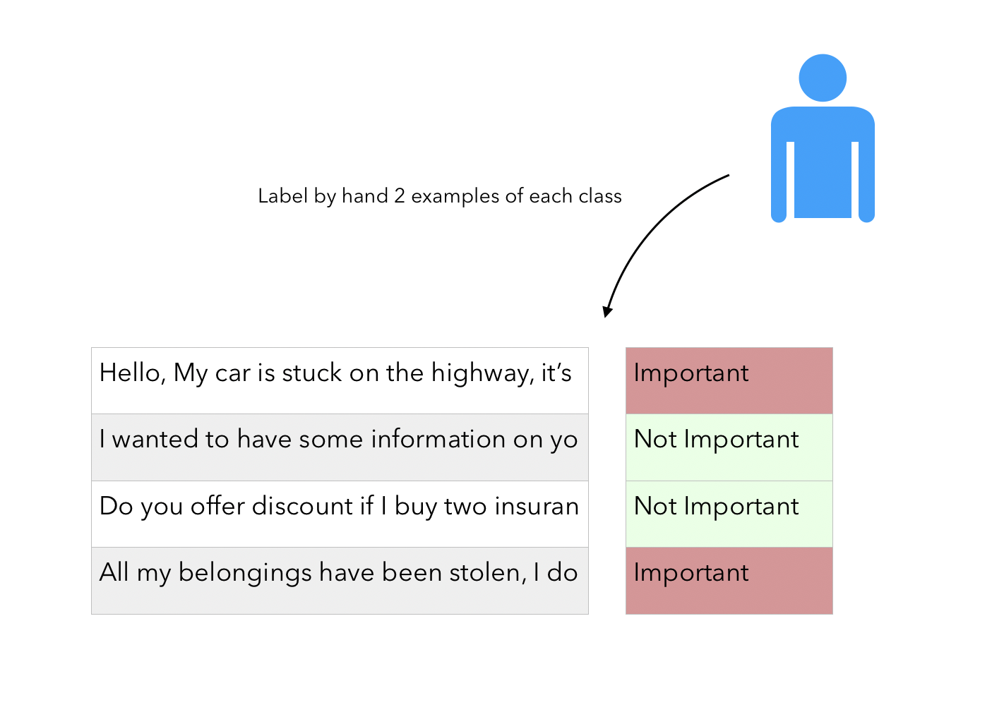
Recall that the fact that there is a “Human in the loop” simply refers to the fact that we have a potentially large corpus of unlabeled data and require the user to label a few examples of each class.

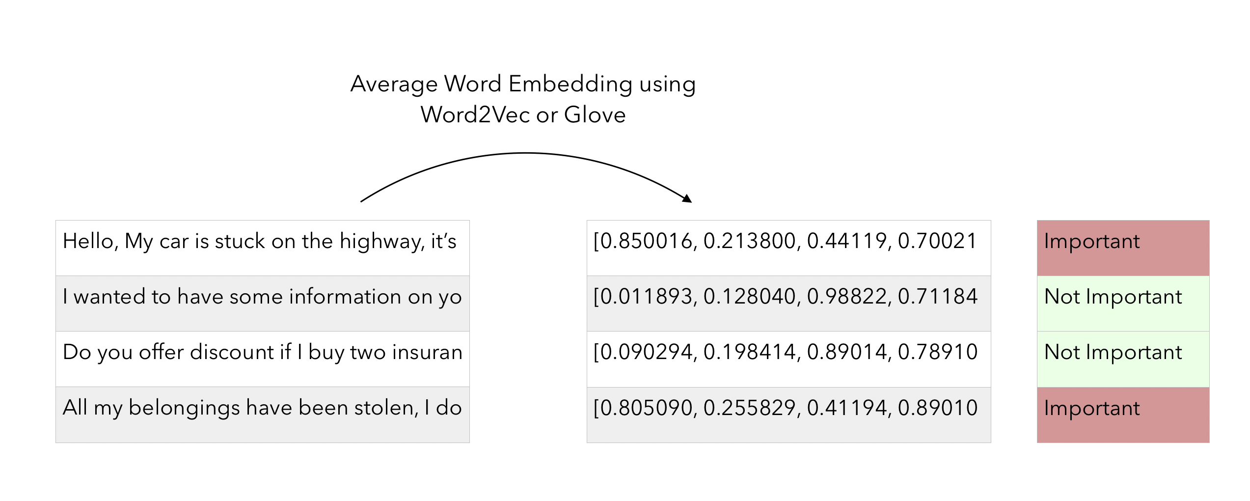
Then, using a pre-trained Word Embedding model (Word2Vec, Glove..), we compute the average embedding of each email / short text in the training examples :

At this point, we compute the avereage embedding for each class :

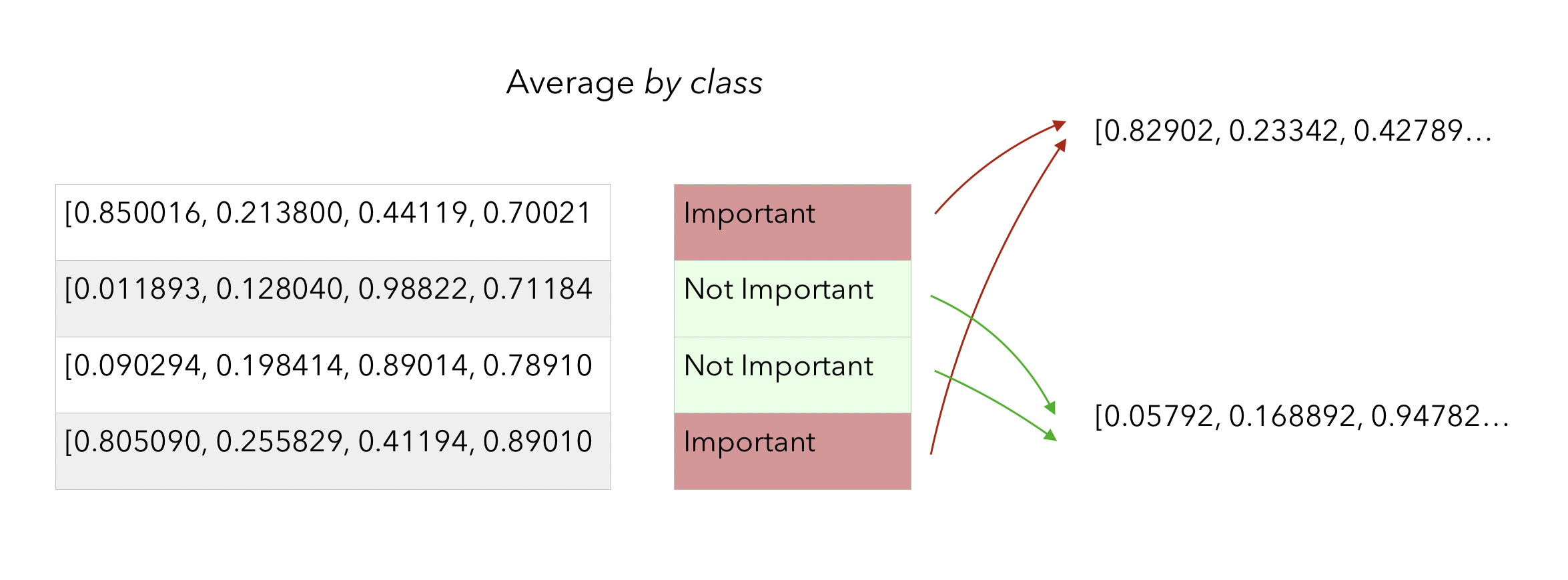
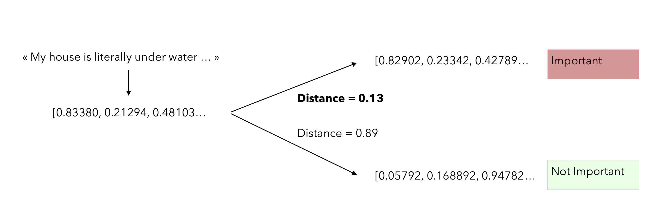
This average embedding per class can be seen as a centroid in a high dimensional space. From that point, when a new observation comes in, we simply have to check how far it is from both centroids, and take the closest. The distance metric used in the paper is the cosine distance :

\[similarity = cos(\theta) = \frac { A \dot B } { \mid \mid A \mid \mid \mid \mid B \mid \mid }\]

Here is the process when a new sentence to classify comes in :

K-NN

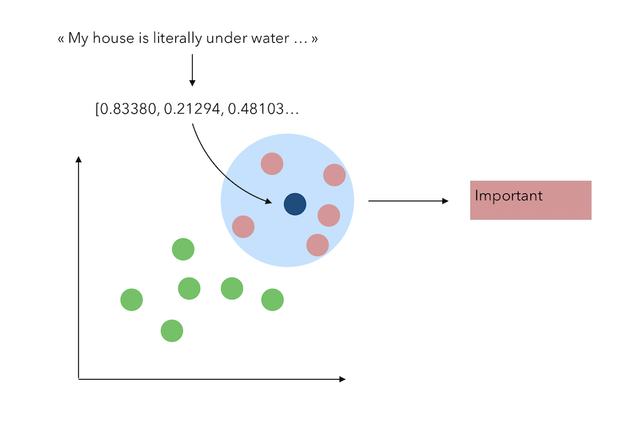
We also explored a K-NN classifier on the pre-trained embeddings. Let’s suppose that the embeding dimension is only 2 (or that we apply a PCA with 2 components) to represent this problem graphically. The classification task with the KNN is the following :

Compared to the previous article, you just need to update your imports :

import pandas as pd
import numpy as np
from random import seed
from random import sample
import random
from random import shuffle
import re

seed(42)
np.random.seed(42)

from sklearn.model_selection import train_test_split
import matplotlib.pyplot as plt

import gensim.downloader as api
from gensim.models.keyedvectors import Word2VecKeyedVectors

from sklearn.decomposition import PCA
from sklearn.metrics import accuracy_score
from scipy import spatial

from sklearn.neighbors import KNeighborsClassifier
from sklearn.ensemble import RandomForestClassifier
from xgboost import XGBClassifier

import nltk
from nltk.corpus import stopwords
from nltk.corpus import wordnet 

And import pre-trained Word2Vec :

model2 = api.load('word2vec-google-news-300')

All the other steps (import the file and clean it) are similar, so I won’t replicate them here.

Data Augmentation

The implementation of the data augmentation is inspired by Easy Data Augmentation (EDA) package, introduced after this paper.

Data augmentation in NLP will be further explored in a dedicated article, but I’ll make a quick summary of the techniques :

• replace words : randomly replace words by a synonym
• random deletion : deletes word of a sentence with a random probability
• random swap : randomly swap words within a sentence
• random insertion : randomly insert a synonym in the sentence

All these techniques simply reply on the idea that we need to create a bit of “noise” in the input data and therefore artificially increase the number of samples we consider. And as we previously saw, this might have a large impact on the final accuracy.

A major question we should now answer is : how many augmented sentences should we create with 1 input sentence? Luckily, the authors of the paper “EDA: Easy Data Augmentation Techniques for Boosting Performance on Text Classification Tasks” provide a summary of the performance gain :

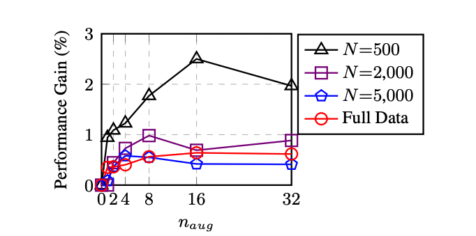
The axis \(n_{aug}\) presents the number of augmented sentences created from a single sentence. Although the authors have not implemented EDA for few-shot learning, with really few training examples (as we have), it seems like 10 to 16 new sentences per input sentence is a good ratio. This should allow us to move from a 5-shot learning to a 50 or even more.

Let’s now implement those data augmentation techniques use the EDA package as a basis:

Replace words

We first need to define a function that finds the synonyms of a word. This relies on synsets, a lexical dictionary that groups synonyms.

def get_synonyms(word):
    
    synonyms = set()
    
    for syn in wordnet.synsets(word): 
        for l in syn.lemmas(): 
            synonym = l.name().replace("_", " ").replace("-", " ").lower()
            synonym = "".join([char for char in synonym if char in ' qwertyuiopasdfghjklzxcvbnm'])
            synonyms.add(synonym) 
    
    if word in synonyms:
        synonyms.remove(word)
    
    return list(synonyms)

Then, create a function to randomly replace a word by one of its synonyms:

stop_words = ['i', 'me', 'my', 'myself', 'we', 'our', 
'ours', 'ourselves', 'you', 'your', 'yours', 
'yourself', 'yourselves', 'he', 'him', 'his', 
'himself', 'she', 'her', 'hers', 'herself', 
'it', 'its', 'itself', 'they', 'them', 'their', 
'theirs', 'themselves', 'what', 'which', 'who', 
'whom', 'this', 'that', 'these', 'those', 'am', 
'is', 'are', 'was', 'were', 'be', 'been', 'being', 
'have', 'has', 'had', 'having', 'do', 'does', 'did',
'doing', 'a', 'an', 'the', 'and', 'but', 'if', 'or',
'because', 'as', 'until', 'while', 'of', 'at', 
'by', 'for', 'with', 'about', 'against', 'between',
'into', 'through', 'during', 'before', 'after', 
'above', 'below', 'to', 'from', 'up', 'down', 'in',
'out', 'on', 'off', 'over', 'under', 'again', 
'further', 'then', 'once', 'here', 'there', 'when', 
'where', 'why', 'how', 'all', 'any', 'both', 'each', 
'few', 'more', 'most', 'other', 'some', 'such', 'no', 
'nor', 'not', 'only', 'own', 'same', 'so', 'than', 'too', 
'very', 's', 't', 'can', 'will', 'just', 'don', 
'should', 'now', '']

def synonym_replacement(words, n):
    
    words = words.split()
    
    new_words = words.copy()
    random_word_list = list(set([word for word in words if word not in stop_words]))
    random.shuffle(random_word_list)
    num_replaced = 0
    
    for random_word in random_word_list:
        synonyms = get_synonyms(random_word)
        
        if len(synonyms) >= 1:
            synonym = random.choice(list(synonyms))
            new_words = [synonym if word == random_word else word for word in new_words]
            num_replaced += 1
        
        if num_replaced >= n: #only replace up to n words
            break

    sentence = ' '.join(new_words)

    return sentence

Finally, apply this function recursively to the existing dataset (append new rows below) :

def iterative_replace(df):
    
    df = df.reset_index().drop(['index'], axis=1)
    index_row = df.index
    df_2 = pd.DataFrame()
    
    for row in index_row:
        for k in range(1,6):
            df_2 = df_2.append({'Text':synonym_replacement(df.loc[row]['Text'], k), 'Label':df.loc[row]['Label']}, ignore_index=True)
    return df_2

Delete words

Let us now build a function to randomly delete words if the value drawn from a uniform distribution is smaller than a threshold :

def random_deletion(words, p):

    words = words.split()
    
    #obviously, if there's only one word, don't delete it
    if len(words) == 1:
        return words

    #randomly delete words with probability p
    new_words = []
    for word in words:
        r = random.uniform(0, 1)
        if r > p:
            new_words.append(word)

    #if you end up deleting all words, just return a random word
    if len(new_words) == 0:
        rand_int = random.randint(0, len(words)-1)
        return [words[rand_int]]

    sentence = ' '.join(new_words)
    
    return sentence

And apply it iteratively :

def iterative_delete(df):
    
    df = df.reset_index().drop(['index'], axis=1)
    index_row = df.index
    df_2 = pd.DataFrame()
    
    for row in index_row:
        df_2 = df_2.append({'Text':random_deletion(df.loc[row]['Text'], 0.25), 'Label':df.loc[row]['Label']}, ignore_index=True)
    return df_2

Random swap

For the random swap, we randomly swap two words in the sentence:

def random_swap(words, n):
    
    words = words.split()
    new_words = words.copy()
    
    for _ in range(n):
        new_words = swap_word(new_words)
        
    sentence = ' '.join(new_words)
    
    return sentence

def swap_word(new_words):
    
    random_idx_1 = random.randint(0, len(new_words)-1)
    random_idx_2 = random_idx_1
    counter = 0
    
    while random_idx_2 == random_idx_1:
        random_idx_2 = random.randint(0, len(new_words)-1)
        counter += 1
        
        if counter > 3:
            return new_words
    
    new_words[random_idx_1], new_words[random_idx_2] = new_words[random_idx_2], new_words[random_idx_1] 
    return new_words

And apply it recursively:

def iterative_swap(df):
    
    df = df.reset_index().drop(['index'], axis=1)
    index_row = df.index
    df_2 = pd.DataFrame()
    for row in index_row:
        df_2 = df_2.append({'Text':random_swap(df.loc[row]['Text'], 2), 'Label':df.loc[row]['Label']}, ignore_index=True)
    return df_2

Random insertion

Finally, regarding the random insertion of synonyms :

def random_insertion(words, n):
    
    words = words.split()
    new_words = words.copy()
    
    for _ in range(n):
        add_word(new_words)
        
    sentence = ' '.join(new_words)
    return sentence

def add_word(new_words):
    
    synonyms = []
    counter = 0
    
    while len(synonyms) < 1:
        random_word = new_words[random.randint(0, len(new_words)-1)]
        synonyms = get_synonyms(random_word)
        counter += 1
        if counter >= 10:
            return
        
    random_synonym = synonyms[0]
    random_idx = random.randint(0, len(new_words)-1)
    new_words.insert(random_idx, random_synonym)

And apply it recursively:

def iterative_insert(df):
    
    df = df.reset_index().drop(['index'], axis=1)
    index_row = df.index
    df_2 = pd.DataFrame()
    
    for row in index_row:
        df_2 = df_2.append({'Text':random_insertion(df.loc[row]['Text'], 2), 'Label':df.loc[row]['Label']}, ignore_index=True)
        
    return df_2

Data Augmentation

Now that the functions are defined, we apply them :

df_replace = iterative_replace(train)
df_delete = iterative_delete(train)
df_swap = iterative_swap(train)
df_insert = iterative_insert(train)

train = pd.concat([train, df_replace, df_delete, df_swap, df_insert], axis=0).reset_index().drop(['index'], axis=1)

The train dataframe used to have shape (8, 2). It now has a shape (72, 2). The data augmentation ratio is 9 here.

Model Performance

Note: The functions return_score and return_score_knn are the same as in the first article.

It is now time to evaluate the performance of the models we previously built (Cosine-based and K-NN).

Cosine Similarity

We can build the prediction :

all_accuracy_aug = {2:[],3:[],4:[],5:[]}
for num_samples in range(1,50):
    for num_cl in range(2, 6):
        all_accuracy_aug[num_cl].append(return_score(num_samples,num_cl))

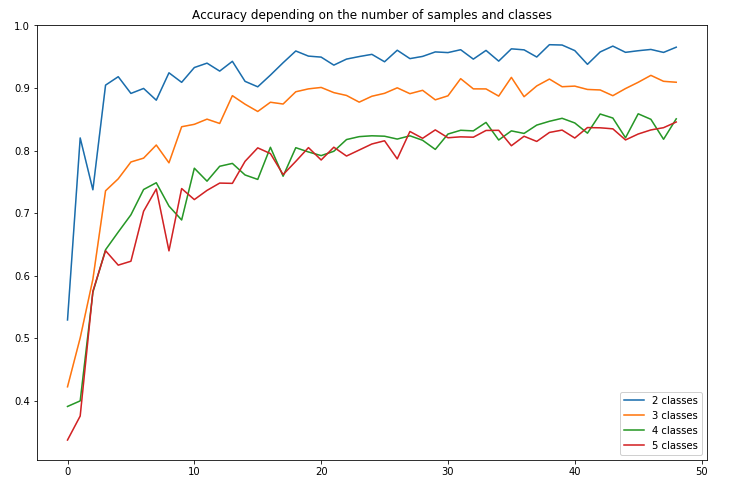
We can plot the accuracy over the number of classes and training samples:

plt.figure(figsize=(12,8))
plt.plot(all_accuracy_aug[2], label="2 classes")
plt.plot(all_accuracy_aug[3], label="3 classes")
plt.plot(all_accuracy_aug[4], label="4 classes")
plt.plot(all_accuracy_aug[5], label="5 classes")
plt.title("Accuracy depending on the number of samples and classes")
plt.legend()
plt.show()

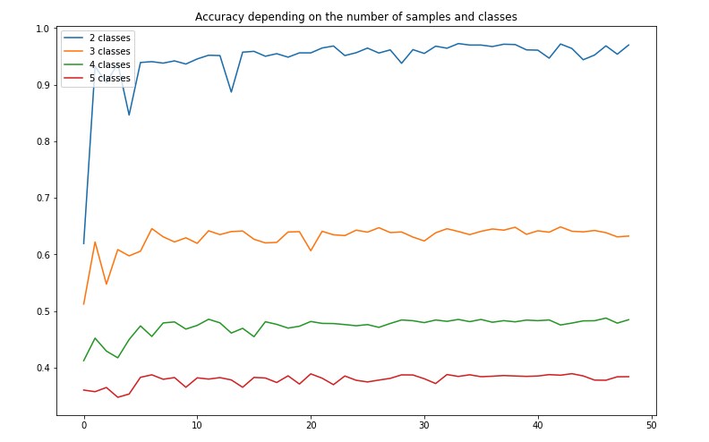
The accuracy does not seem to improve significantly. We can now do the same for the K-NN approach.

K-NN approach

First, compute the accuracy for each number of sample and number of classes:

all_accuracy_knn_aug = {2:[],3:[],4:[],5:[]}
for num_samples in range(1,50):
    for num_cl in range(2, 6):
        all_accuracy_knn_aug[num_cl].append(return_score_knn(num_samples,num_cl))

Then, plot the accuracy:

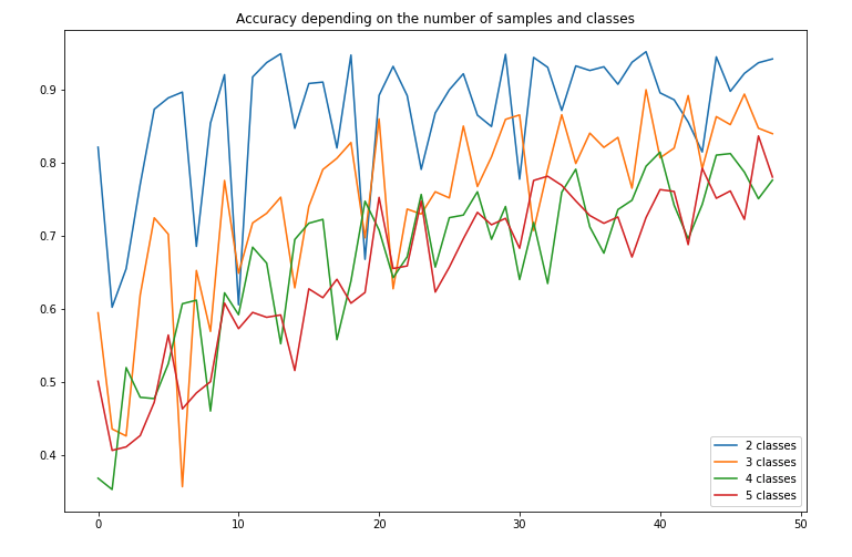
The accuracy remains quite high, but seems to suffer from a large volatility depending on the number of samples we take. A performance summary is presented here:

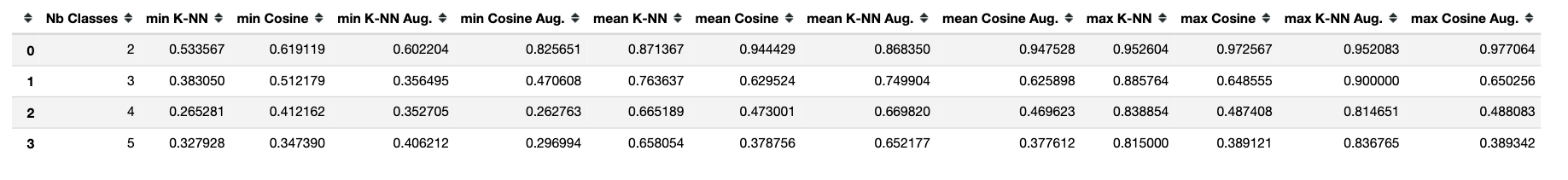
Since the volatility seems to be one of the main issues here, could more powerful models help leverage the data augmentation?

Better Model

In terms of model, I chose to explore both XGBoost and a Random Forest Classifier. The Random Forest seemed to outperform the XGBoost with a lower training time, and I will present the approach for this model only (although it can be easily replicated for all models).

Start by re-defining a return_score function in which you change the classifier to Random Forest :

def return_score_rf(sample_size, num_classes):
    
    train, test = gen_sample(sample_size, num_classes)
    
    X_train = train['Text']
    y_train = train['Label'].values
    X_test = test['Text']
    y_test = test['Label'].values

    X_train_mean = X_train.apply(lambda x : transform_sentence(x, model2))
    X_test_mean = X_test.apply(lambda x : transform_sentence(x, model2))

    X_train_mean = pd.DataFrame(X_train_mean)['Text'].apply(pd.Series)
    X_test_mean = pd.DataFrame(X_test_mean)['Text'].apply(pd.Series)
        
    clf = RandomForestClassifier(n_estimators=150)
    clf.fit(X_train_mean, y_train)
    
    y_pred = clf.predict(X_test_mean)
    
    return accuracy_score(y_pred, y_test)

Then, compute the accuracy on the test set for all class and train set samples:

all_accuracy_rf_aug = {2:[],3:[],4:[],5:[]}
for num_samples in range(1,50):
    for num_cl in range(2, 6):
        all_accuracy_rf_aug[num_cl].append(return_score_rf(num_samples,num_cl))

Finally, plot the results :

plt.figure(figsize=(12,8))
plt.plot(all_accuracy_rf_aug[2], label="2 classes")
plt.plot(all_accuracy_rf_aug[3], label="3 classes")
plt.plot(all_accuracy_rf_aug[4], label="4 classes")
plt.plot(all_accuracy_rf_aug[5], label="5 classes")
plt.title("Accuracy depending on the number of samples and classes")
plt.legend()
plt.show()

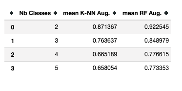
The Random Forest seems to be largely outperforming the K-NN Classifier here:

Conclusion

Overall, throughout this 2-parts article, we saw different approaches that rely on trained models. The cosine similarity approach is still a good choice for binary classification with really few examples (less than 3). However, with only 8 training samples per class, we are able to outperform the 5-class performance of the cosine model by more than 40% thanks to the Random Forest Classifier. The data augmentation allows us to apply models that are a bit more complex by multiplying the number of training samples by a factor of 9 here.

The final accuracy is quite impressive, close to 80% for 3, 4 or 5 classes, and more than 95% for 2 classes when we have only 8 training samples per class.

The pre-trained model (Word2Vec) was moreover trained on a general corpus, whereas our classification task was focused on Stackoverflow questions. We could also leverage the fact that some supervised learning problem would allow us to pre-train a model on a corpus that is closer to our task here.

I hope you found this article interesting. Please leave a comment if you have any question, or if you implement similar solutions and would like to discuss your results.