
I recently came across a good blog post article published by Nicolas Thiebaut right here. This article addresses the task of classifying texts when we have few training examples. I started to read some litterature on this topic, and it’s impressive to notice that you can count on your fingertips the number of articles that adress this topic.
Problem definition
This kind of problem is however easily encountered. Suppose that your company gets customer emails, that are not labeled. You work in the data science department, and you want to automatically label the emails by saying whether they are important or not. It’s a simple binary classification. Labeling data might be incredibly long and cumbersome. You might even never reach enough labeled data for classical NLP classification tasks.
This kind of problem needs to be adressed in another way. Let’s start by defining scenarios that might occur :
- Zero-shot learning : you have some labeled observations per classes, but some classes don’t have observations. It’s a tricky case that we won’t address in this article
- One-shot learning : we have one labeled observation per class
- Few-shot learning : we have few observations per class
It’s now much easier to think of your email classification as a One-Shot or Few-Shot learning problem. Indeed, you could easily ask a business user to classify, say 10 emails, 5 important, and 5 not important, and take that as input data.
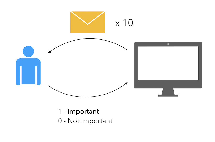
The data labeling would take 5 minutes at most. Now, the question becomes : what the hell can I do with 10 training examples?
Solutions
Few shot learning is largely studied in the field of computer vision. Papers published in this field quite often rely on Siamese Networks. A typical application of such problem would be to build a Face Recognition algorithm. You have 1 or 2 pictures per person, and need to assess who is on the video the camera is filming. However, in the domain of Natural Language Processing, this problem is less common.
In most few shot learning problems, there is a notion of distance that arises at some point. In Siamese networks, we want to minimize the distance between the anchor and the other positive example, and maximize the distance between the anchor and negative example.
I have seen several approaches to few shot learning in recent papers :
- either use a Siamese Network based on LSTMs rather than CNNs, and use this for One-shot learning
- learn word embeddings in one-shot or few-shot and classify on top
- or use a pre-trained word / document embedding network, and build a metric on top
We will focus on the last solution. This article is an implementation of a recent paper, Few-Shot Text Classification with Pre-Trained Word Embeddings and a Human in the Loop by Katherine Bailey and Sunny Chopra Acquia. A simple presentation of the paper can paper can be found here.
Few-Shot with Human in the Loop
Concept
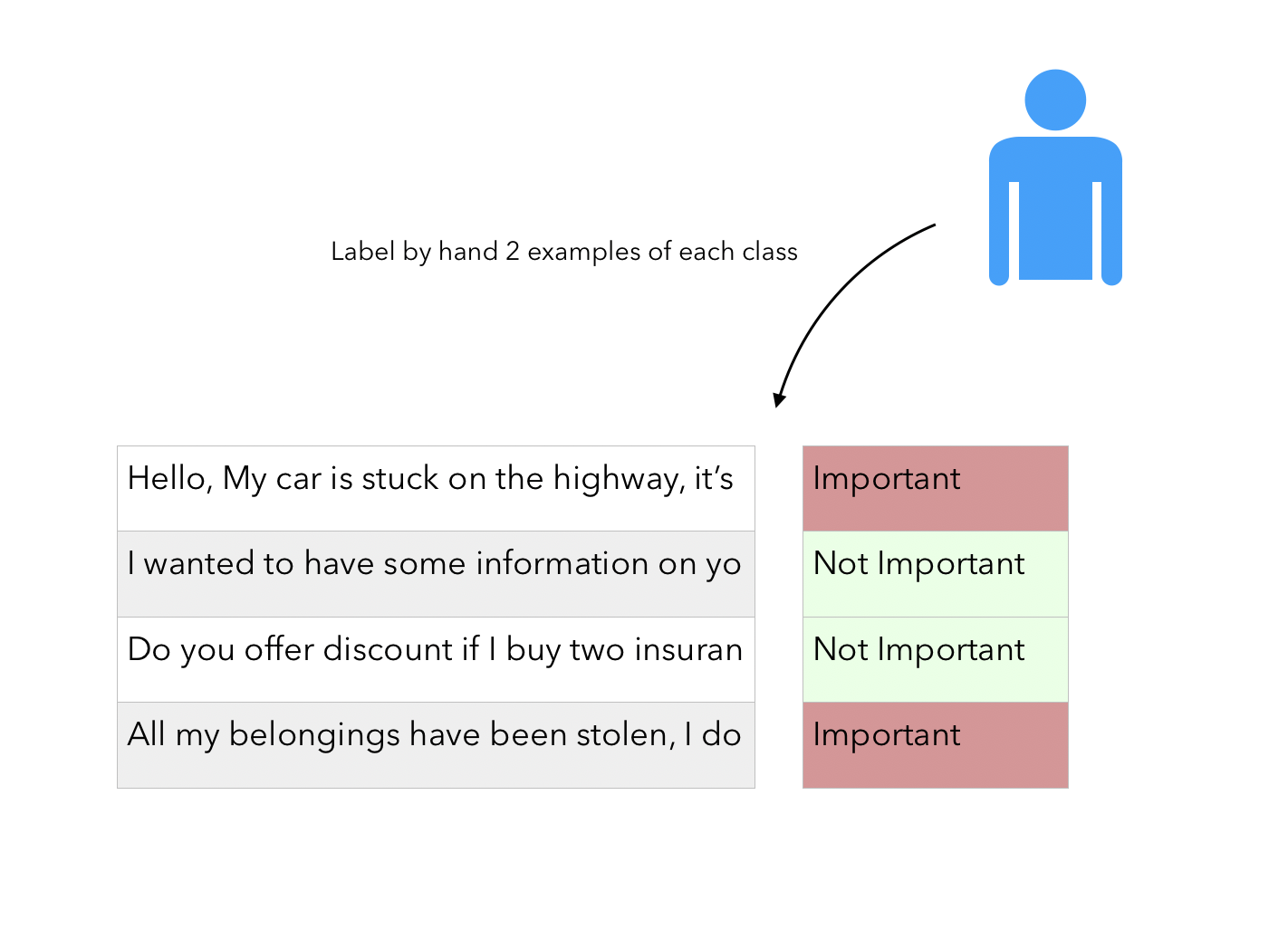
Let’s start by formalizing the main idea behind the paper. The fact that there is a “Human in the loop” simply refers to the fact that we have a potentially large corpus of unlabeled data and require the user to label a few examples of each class.
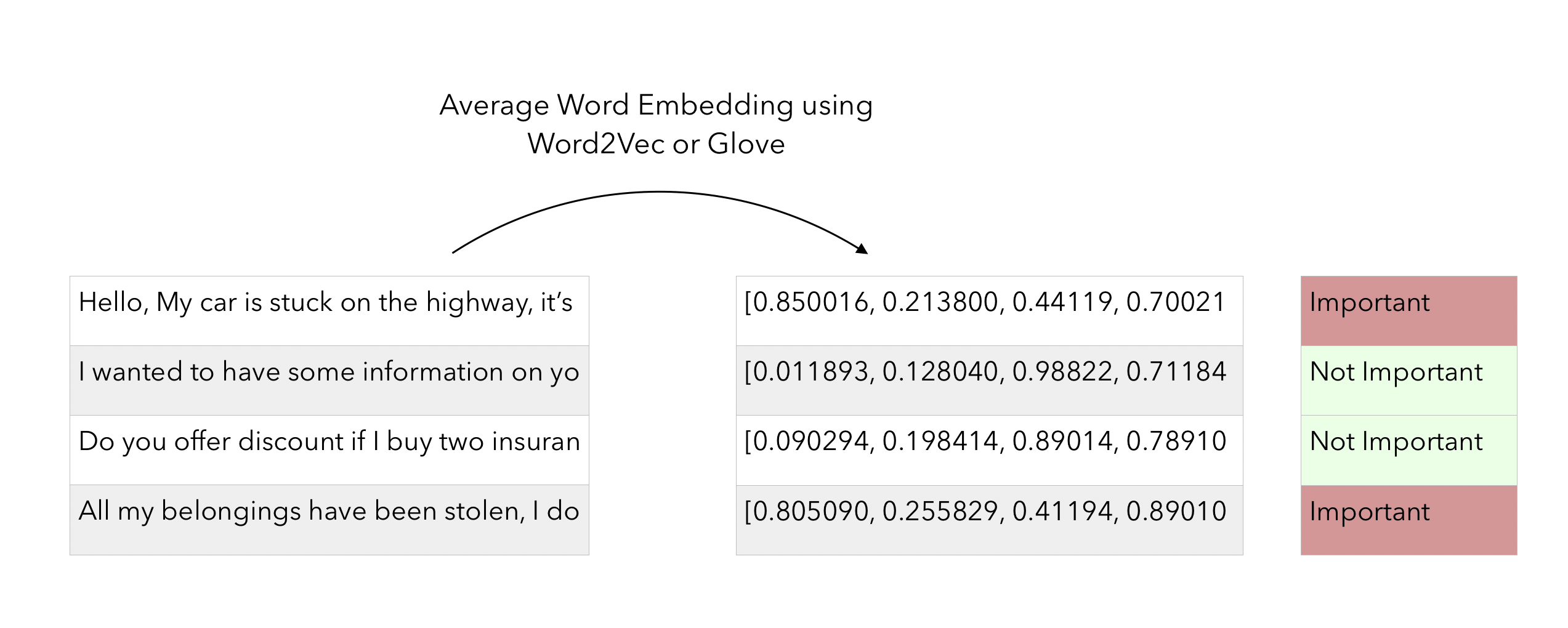
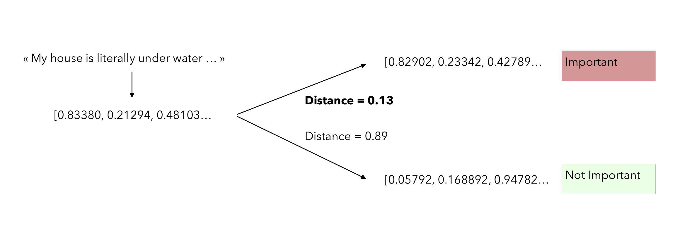
Then, using a pre-trained Word Embedding model (Word2Vec, Glove..), we compute the average embedding of each email / short text in the training examples :
At this point, we compute the avereage embedding for each class :
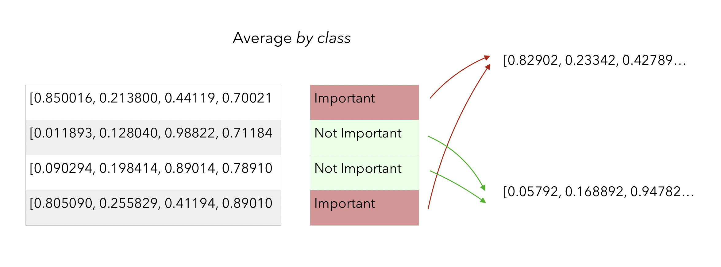
This average embedding per class can be seen as a centroid in a high dimensional space. From that point, when a new observation comes in, we simply have to check how far it is from both centroids, and take the closest. The distance metric used in the paper is the cosine distance :
\[similarity = cos(\theta) = \frac { A \dot B } { \mid \mid A \mid \mid \mid \mid B \mid \mid }\]Here is the process when a new sentence to classify comes in :
Implementation
Start by importing the following packages :
import pandas as pd
import numpy as np
from random import seed
from random import sample

seed(42)
np.random.seed(42)

from sklearn.model_selection import train_test_split
import matplotlib.pyplot as plt

import gensim.downloader as api
from gensim.models.keyedvectors import Word2VecKeyedVectors

from sklearn.decomposition import PCA
from sklearn.metrics import accuracy_score
from scipy import spatial

from nltk.corpus import stopwords
We will use pre-trained models from Gensim :
#model = api.load('glove-twitter-25') Not used
model2 = api.load('word2vec-google-news-300')
As you can see, I have tried this exercise with both Glove and Word2Vec, and chose to stick to Word2Vec. Let us now load a dataset that would suit. I have found a short text classification dataset from StackOverflow, where the corresponding categories are actually the language/forum category the question falls into.
You can download it here. I called it “Stack” for what comes next, since the first step was to concatenate the texts and the labels (skipped here to keep it short) :
df = pd.read_csv("stack.csv")
df.head()
| Text | Label | |
| 0 | How do I fill a DataSet or a DataTable from a … | 18 |
| 1 | How do you page a collection with LINQ? 18 | |
| 2 | Best Subversion clients for Windows Vista (64bit) | 3 |
| 3 | Best Practice: Collaborative Environment, Bin … | 3 |
| 4 | Visual Studio Setup Project - Per User Registr… | 7 |
We can now clean the texts in order to keep only the characters :
def get_only_chars(line):

    clean_line = ""

    line = line.replace("’", "")
    line = line.replace("'", "")
    line = line.replace("-", " ") #replace hyphens with spaces
    line = line.replace("\t", " ")
    line = line.replace("\n", " ")
    line = line.lower()

    for char in line:
        if char in 'qwertyuiopasdfghjklzxcvbnm ':
            clean_line += char
        else:
            clean_line += ' '

    clean_line = re.sub(' +',' ',clean_line) #delete extra spaces
    if clean_line[0] == ' ':
        clean_line = clean_line[1:]
    return clean_line
Then, apply the function to the text column :
df['Text'] = df['Text'].apply(lambda x: get_only_chars(x))
Then, there are 2 variables which we’ll have to control :
- the number of classes we consider (since the dataset has many classes)
- the number of labeled sampled we’ll require from the user
We set the by default to :
num_classes = 2
sample_size = 3
We then must generate samples that contain \(K = 3\) training samples per class, and \(M = 2\) classes :
# Generate samples that contains K samples of each class

def gen_sample(sample_size, num_classes):

    df_1 = df[(df["Label"]<num_classes + 1)].reset_index().drop(["index"], axis=1).reset_index().drop(["index"], axis=1)
    train = df_1[df_1["Label"] == np.unique(df_1['Label'])[0]].sample(sample_size)

    train_index = train.index.tolist()

    for i in range(1,num_classes):
        train_2 = df_1[df_1["Label"] == np.unique(df_1['Label'])[i]].sample(sample_size)
        train = pd.concat([train, train_2], axis=0)
        train_index.extend(train_2.index.tolist())

    test = df_1[~df_1.index.isin(train_index)]

    return train, test
Apply that to the dataframe :
train, test = gen_sample(sample_size, num_classes)

X_train = train['Text']
y_train = train['Label'].values
X_test = test['Text']
y_test = test['Label'].values
train now contains only 6 observations, 3 from each class :
| Text | Label | |
| 1421 | Lighttp and wordpress URL rewrite | 1 |
| 1275 | wordpress plug-ins, themes and widgets tips … | 1 |
| 1638 | Is there an easier way to add menu items to a … | 1 |
| 735 | Oracle deadlock detection tool | 2 |
| 1074 | Index not used due to type conversion? | 2 |
| 311 | UTF 8 from Oracle tables | 2 |
At that point, we need to get the aveage embeddings by first getting the token id in the model vocabulary, and then getting the corresponding word embedding, before finally average over the whole sentence.
# Text processing (split, find token id, get embedidng)
def transform_sentence(text, model):

    """
    Mean embedding vector
    """

    def preprocess_text(raw_text, model=model):

        """
        Excluding unknown words and get corresponding token
        """

        raw_text = raw_text.split()

        return list(filter(lambda x: x in model.vocab, raw_text))

    tokens = preprocess_text(text)

    if not tokens:
        return np.zeros(model.vector_size)

    text_vector = np.mean(model[tokens], axis=0)

    return np.array(text_vector)
Apply this to both the train and the test :
X_train_mean = X_train.apply(lambda x : transform_sentence(x, model2))
X_test_mean = X_test.apply(lambda x : transform_sentence(x, model2))

X_train_mean = pd.DataFrame(X_train_mean)['Text'].apply(pd.Series)
X_test_mean = pd.DataFrame(X_test_mean)['Text'].apply(pd.Series)
We will now use cosine similarity between the embeddings of the text to classify and the average embeddings of all classes. A new example therefore belongs to the class it is the closest to.
# Use cosine similarity to find closest class
def classify_txt(txt, mean_embedding):

    best_dist = 1
    best_label = -1

    for cl in range(num_classes):

        dist = spatial.distance.cosine(transform_sentence(txt, model2), mean_embedding[cl])

        if dist < best_dist :
            best_dist = dist
            best_label = cl+1

    return best_label
The point in doing all this is to see how the classification accuracy reacts to the number of classes and to the number of training examples. Let us now create a function that gathers all the previous steps and iterates on the test set to compute the accuracy :
# Process text and predict on the test set
def return_score(sample_size, num_classes):

    train, test = gen_sample(sample_size, num_classes)

    X_train = train['Text']
    y_train = train['Label'].values
    X_test = test['Text']
    y_test = test['Label'].values

    X_train_mean = X_train.apply(lambda x : transform_sentence(x, model2))
    X_test_mean = X_test.apply(lambda x : transform_sentence(x, model2))

    X_train_mean = pd.DataFrame(X_train_mean)['Text'].apply(pd.Series)
    X_test_mean = pd.DataFrame(X_test_mean)['Text'].apply(pd.Series)

    mean_embedding = {}
    for cl in range(num_classes):
        mean_embedding[cl] = np.mean((X_train_mean[y_train == cl + 1]), axis=0)

    y_pred = [classify_txt(t, mean_embedding) for t in test['Text'].values]

    return accuracy_score(y_pred, y_test)
Now, we will iterate on the number of classes (between 2 and 7) and the number of samples (between 1 andd 50). We will consider that labeling more than 50 training examples per class is too long.
all_accuracy = {2:[],3:[],4:[],5:[],6:[],7:[]}

for num_samples in range(1,50):
    for num_cl in range(2, 7):
        all_accuracy[num_cl].append(return_score(num_samples,num_cl))
This will take several minutes to run. Once we are done, we can plot the accuracy for each number of class (the color) depending on the number of training examples (the y-axis) :
plt.figure(figsize=(12,8))
plt.plot(all_accuracy[2], label="2 classes")
plt.plot(all_accuracy[3], label="3 classes")
plt.plot(all_accuracy[4], label="4 classes")
plt.plot(all_accuracy[5], label="5 classes")
plt.plot(all_accuracy[6], label="6 classes")
plt.axvline(7, c='black', alpha=0.5)
plt.title("Accuracy depending on the number of samples and classes")
plt.legend()
plt.show()
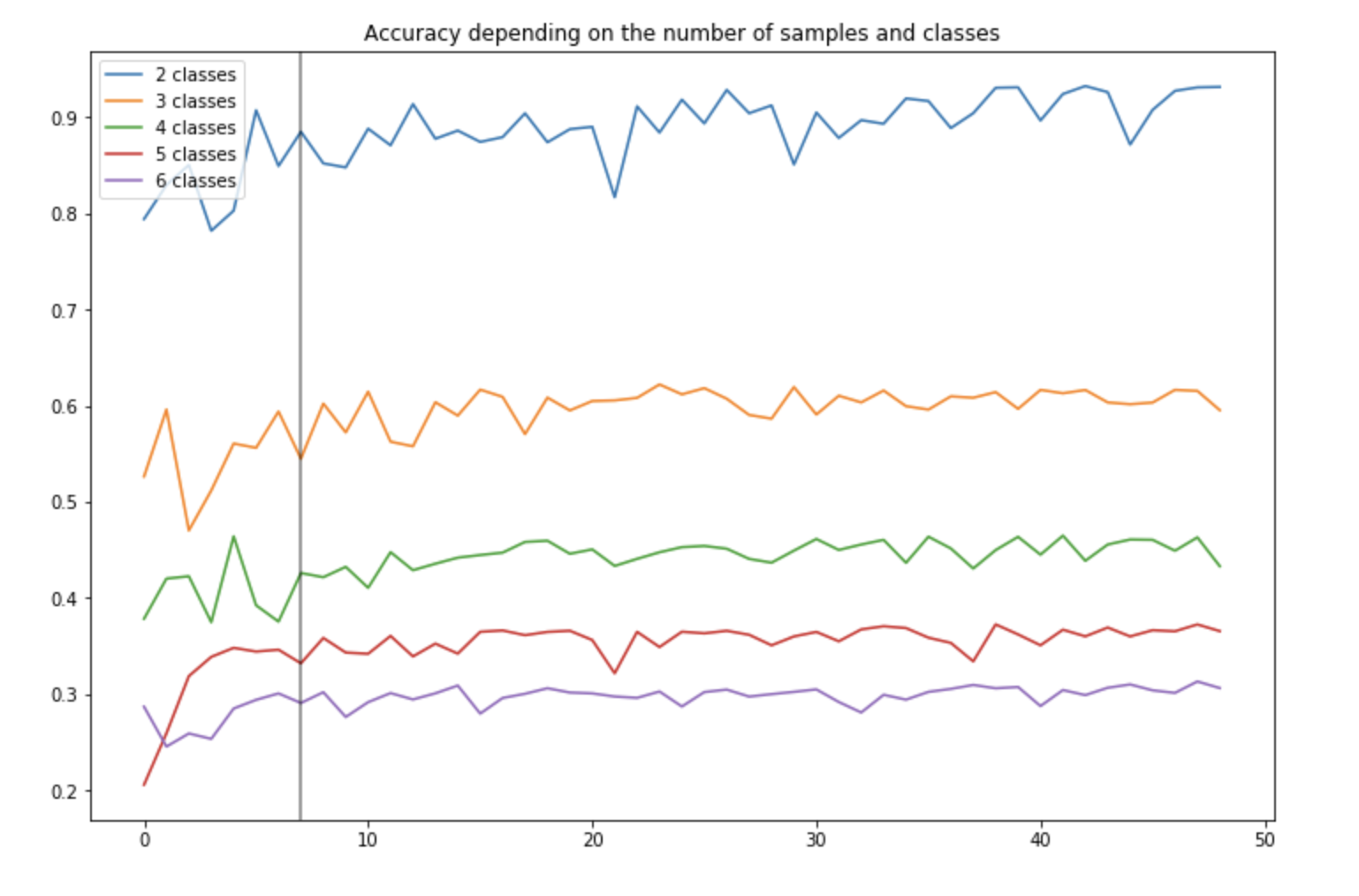
For 2 classes, we rapidly reach an accuracy of about 90%. Notice how the accuracy decreases with the number of classes, but remain above the “random” allocation threshold. For 4 classes, the accuracy is indeed of 40%, and remains above 25% if we were to classify randomly.
The results are quite encouraging, but the approach of distance metric is quite restrictive since it relies on comparing the embedding of a sentence (which is itself an average of word embeddings), with the average of the embedding of all training examples within a class. That makes a lot of averages. Couldn’t we go a little further and avoid averaging the embedding of the training examples ?
Pre-trained Word2Vec and K-NN
We are going to use the same logic as defined above. However, instead of averaging the embeddings for each class, we will keep the embeddings as separate observations. Instead, once a new observation comes in, we will apply a K-Nearest Neighbors classifier for the classification task.
Let’s suppose that the embeding dimension is only 2 (or that we apply a PCA with 2 components) to represent this problem graphically. The classification task with the KNN is the following :
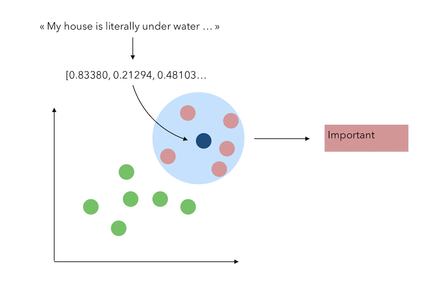
One important note about the parameter choice for the K-NN : I think that looking at as many neighbors as we have of training samples per class is intuitive. Say if we have 5 samples per class, and we must classify a new observation, then if the classes are different enough, we should be able to have the 5 neighbors with the same label. If we were to set this number of neighbors to consider manually, we would risk to take too many points into consideration.
Let’s modify the return_score function :
from sklearn.neighbors import KNeighborsClassifier

def return_score(sample_size, num_classes):

    train, test = gen_sample(sample_size, num_classes)

    X_train = train['Text']
    y_train = train['Label'].values
    X_test = test['Text']
    y_test = test['Label'].values

    X_train_mean = X_train.apply(lambda x : transform_sentence(x, model2))
    X_test_mean = X_test.apply(lambda x : transform_sentence(x, model2))

    X_train_mean = pd.DataFrame(X_train_mean)['Text'].apply(pd.Series)
    X_test_mean = pd.DataFrame(X_test_mean)['Text'].apply(pd.Series)

    clf = KNeighborsClassifier(n_neighbors=sample_size, p=2)
    clf.fit(X_train_mean, y_train)

    y_pred = clf.predict(X_test_mean)

    return accuracy_score(y_pred, y_test)
And run the same loop as above :
all_accuracy_knn = {2:[],3:[],4:[],5:[],6:[],7:[]}

for num_samples in range(1,50):

    for num_cl in range(2, 7):

        all_accuracy_knn[num_cl].append(return_score(num_samples,num_cl))
Then, plot the results :
plt.figure(figsize=(12,8))
plt.plot(all_accuracy_knn[2], label="2 classes")
plt.plot(all_accuracy_knn[3], label="3 classes")
plt.plot(all_accuracy_knn[4], label="4 classes")
plt.plot(all_accuracy_knn[5], label="5 classes")
plt.plot(all_accuracy_knn[6], label="6 classes")
plt.title("Accuracy depending on the number of samples and classes")
plt.legend()
plt.show()
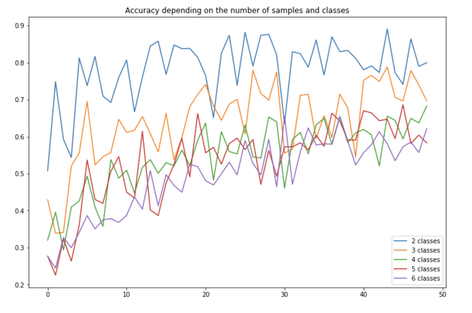
When we have really few training samples (less than 10), the cosine-based approach seems to outperform the K-NN. However, once we consider more than 10 training samples, the accuracy with 4 classes improves from 40% to 67% !
Summary
We can now group this into a summary table :
df_results = pd.DataFrame({
    'Nb Classes':[2,3,4,5],
    'min K-NN':[min(all_accuracy_knn[2]),
        min(all_accuracy_knn[3]),
        min(all_accuracy_knn[4]),
        min(all_accuracy_knn[5])],
    'min Cosine':[min(all_accuracy[2]),
        min(all_accuracy[3]),
        min(all_accuracy[4]),
        min(all_accuracy[5])],
    'mean K-NN':[np.mean(all_accuracy_knn[2]),
        np.mean(all_accuracy_knn[3]),
        np.mean(all_accuracy_knn[4]),
        np.mean(all_accuracy_knn[5])],
    'mean Cosine':[np.mean(all_accuracy[2]),
        np.mean(all_accuracy[3]),
        np.mean(all_accuracy[4]),
        np.mean(all_accuracy[5])],
    'max K-NN':[max(all_accuracy_knn[2]),
        max(all_accuracy_knn[3]),
        max(all_accuracy_knn[4]),
        max(all_accuracy_knn[5])],
    'max Cosine':[max(all_accuracy[2]),
        max(all_accuracy[3]),
        max(all_accuracy[4]),
        max(all_accuracy[5])]
    })
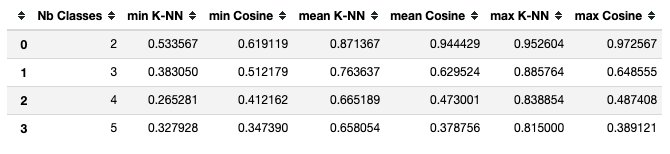
On average, the K-NN is better if there are more than 2 classes, and a sufficient amount of training samples.
Conclusion
We have covered in this article a really simple implementation of Few-Shot Text Classification with Pre-Trained Word Embeddings and a Human in the Loop. This paper is interesting since it addresses a concrete problem you might encounter. The solution proposed by the authors (although I skipped the PCA part) seems to perform well if we have few classes and few trainign examples. On the other hand, the extension that I developped with K-NNs outperforms the solution once we consider more samples and more classes. There seems to be a trade-off to make here when choosing the right approach.
I hope this article was interesting. If you implement it on your own, please share your results and improvements of the current solution !