
In this article, we’ll cover the main functions to conduct a statistical analysis. I’m working on a sample data set that describes the salaries of employees depending on several features.
I. Data exploration
The file I’m working on comes with a small description DES. The description of the data is the following.
wage      educ      exper     tenure    nonwhite  female    married   numdep
smsa      northcen  south     west      construc  ndurman   trcommpu  trade
services  profserv  profocc   clerocc   servocc   lwage     expersq   tenursq

Obs:   526

1. wage                     average hourly earnings
2. educ                     years of education
3. exper                    years potential experience
4. tenure                   years with current employer
5. nonwhite                 =1 if nonwhite
6. female                   =1 if female
7. married                  =1 if married
8. numdep                   number of dependents
9. smsa                     =1 if live in SMSA
10. northcen                 =1 if live in north central U.S
11. south                    =1 if live in southern region
12. west                     =1 if live in western region
13. construc                 =1 if work in construc. indus.
14. ndurman                  =1 if in nondur. manuf. indus.
15. trcommpu                 =1 if in trans, commun, pub ut
16. trade                    =1 if in wholesale or retail
17. services                 =1 if in services indus.
18. profserv                 =1 if in prof. serv. indus.
19. profocc                  =1 if in profess. occupation
20. clerocc                  =1 if in clerical occupation
21. servocc                  =1 if in service occupation
22. lwage                    log(wage)
23. expersq                  exper^2
24. tenursq                  tenure^2
The first step is to load the data set in our path :
wage1=load('WAGE1.raw')
[n,k]=size(wage1)
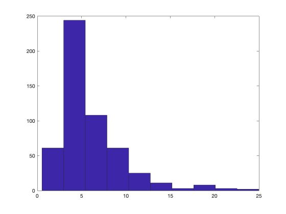
Then, we’ll plot a histogram of hourly salaries :
hist(wage1(:,1))
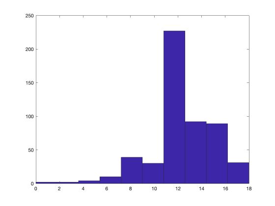
Now, let’s plot the histogram for the number of years of education.
We can take a look at the mean of each feature :
mean(wage1(:,:))'
ans =

5.8961
12.5627
17.0171
5.1046
0.1027
...
We can also take a look at other descriptive statistics :
std(wage1(:,:))'
min(wage1)'
max(wage1)'
cov(wage1)'
corrcoef(wage1(:,:))'
II. Linear regression
Compute coefficients
We now want to assess the effect of columns 2, 3 and 4 (education, experience, years with current employer) on the salary.
\[y_i = \beta_0 + \beta_1 * {x_1}_i + \beta_2 * {x_2}_i + \beta_3 * {x_3}_i + u_i\]y=wage1(:,1)
X=[ones(n,1),wage1(:,[2,3,4])]
We can compute the Beta coefficients and the residuals :
beta=inv(X'*X)*X'*y
u=y-X*beta
The coefficients are the following :
beta =

-2.8727
0.5990
0.0223
0.1693
The first coefficient is constant. Then, the model indicates that an additional year of education should increase the hourly salary by 0.60$.
Residuals
Effect of each feature individually
We can also plot a histogram of the residuals. The distribution of the residual appears to be close to a normal one.
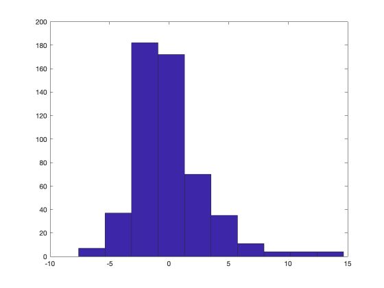
We can decide to remove outliers above 5 for example :
indices = find(u>2.5);
u(indices) = [];
hist(u)
Test hypothesis
Are the coefficients significant?
To assess the significance of each estimator, we need to estimate their standard deviation.
sig2=u'*u/(n-4)
std=sqrt(diag(sig2*inv(X'*X)))
Then, we can easily compute the test statistic :
t = beta./std
t =

-5.6300
16.6857
2.6471
11.1725
What should we compare the test statistics? Well, to the critical value! For example, since we estimate 4 parameters, the 95% critical value is :
C1 = tinv(0.95, n-4)
C1 =

1.6478
The T-stats are all greater than the critical value. For this reason, we reject the hypothesis \(H_0\) that the variables have no impact on the output.
Effect of a single feature
If we are interested in the effect of a single feature, we can specify a value for its effect for example.
t_educ = (beta(2)-0.1)/std(2)
Effect of each feature on log(wage)
Testing the effect of the features on the log(wage) is a way to assess their importance in terms of the percentage change.
y=log(wage1(:,1))
beta=inv(X'*X)*X'*y
std=sqrt(diag(sig2*inv(X'*X)))
t = beta./std
Test is 2 features have the same effect
Now, let’s test the following hypothesis: the effect of education is the same as the effect of professional experience. This can be rewritten as : \(H_0 : \beta_2 = \beta_3\) . However, estimating the variance of \(\beta_2 - \beta_3\) to build the test hypothesis would be challenging. We can apply a simple trick by building a new feature as the sum of the 2 features to test.
First of all, append the new feature to the model :
capitaltot = X(:,2) + X(:,3)
This introduces some multicolinearity which we should control by removing \(X_3\) :
X=[X(:,[1,2,4]),capitaltot];
y=log(wage1(:,1))
We can run the test : \(H_0 : \beta_4 = 0\)
beta=inv(X'*X)*X'*y
std=sqrt(diag(sig2*inv(X'*X)))
t = beta(4)/std(4)
This heads :
t =

0.4883
The T-test is smaller than the critical value. For this reason, we cannot reject the hypothesis that the effect in the percentage of education is the same as the one of professional experience.
Fisher Test for joint hypothesis
Let us now consider the hypothesis : \(H_0 : \beta_2 = 0, \beta_3 = 0\) . In such case, we should not apply 2 independent tests, since we are interested in the overall hypothesis.
We need to define a non-constrained model, a constrained model and test the difference between those two models.
% non-constrained model
X0=[ones(n,1),wage1(:,[2,3,4])]
y0=log(wage1(:,1))
beta0=inv(X0'*X0)*X0'*y0
u0=y0-X0*beta0
SSR0=u0'*u0
% model contraint
X1=[ones(n,1),wage1(:,[4])]
y1=log(wage1(:,1))
beta1=inv(X1'*X1)*X1'*y1
u1=y1-X1*beta1
SSR1=u1'*u1
The Fisher F-Stat is defined as :
\[\hat{F}_j = \frac { {SSR}_1 - {SSR}_0 } { {SSR}_0} \frac {n - K} {2}\]Where K is the number of variables included in the non-constrained model (4 here).
K = 4
F = (SSR1-SSR0)/(SSR0) * (n-K)/2
This heads :
F =

80.1478
Interaction effect
Let’s define new variables :
X=wage1
educ=X(:,2)
exper=X(:,3)
tenure=X(:,4)
female=X(:,6)
married=X(:,7)
marrmale = (1-female).*married
marrfem = female.*married
singfem=female.*(1-married)
We create interaction variables :
- effect of a married male
- effect of a married female
- effect of a single female
The base case is a single male. We can define test statistics on those variables as we did above.
**Conclusion **: This was a quick introduction to Matlab. I hope you found it useful. Don’t hesitate to drop a comment if you have a question.