
So far, with the linear model, we have seen how to predict continuous variables. What happens when you want to classify with a linear model?
Linear Probability Model
Suppose that our aim is to do binary classification : \(y_i = \{0,1\}\). Let’s consider the model :
\[y = \beta_0 + \beta_1 X_1 + ... + \beta_k X_k + u\]Where \(E(u \mid X_1, ... X_k) = 0\). How can we perform binary classification with this model? Let’s start with a dataset in which you have binary observations and you decide to fit a linear regression on top of it.
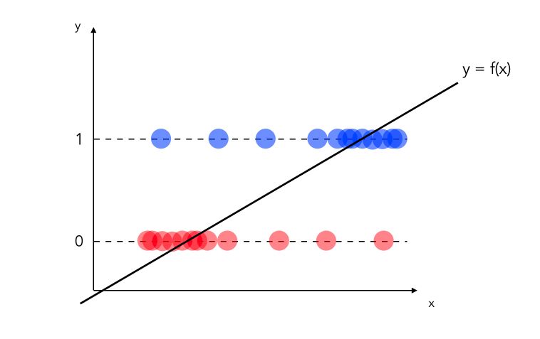
Statistically speaking, the model above is incorrect :
- we would need to define a threshold under which we classify as 0, and above which we classify 1
- what if the values are greater than 1? Or smaller than 0?
- …
Linear probability model has however one main advantage: the coefficients remain easily interpretable!
\[\Delta P(Y=1 \mid X) = \beta_j \Delta X_j\]In other words, the impact of a coefficient can be measured as a contribution percentage to the final classification. Overall, this model needs to be adjusted/transformed to throw the predicted between values between 0 and 1. This is the main idea of logistic regression!
Logistic Regression
We are now interested in \(P(Y=1 \mid X) = P(Y=1 \mid X_1, X_2, .. X_k) = G(\beta_0 + \beta_1 X_1 + ... + \beta_k X_k)\). As you might guess, the way we define \(G\) will define the way we make our mapping.
- If \(G\) is linear, this is obviously the linear regression
- If \(G\) is a sigmoid : \(G(z) = \frac {1} {1 + e^{-z}}\), then the model is a logistic regression
- If \(G\) is a normal transformation \(G(z) = \Phi(z)\), then the model is a probit regression
In this article, we’ll focus on logistic regression.
Sigmoid and Logit transformations
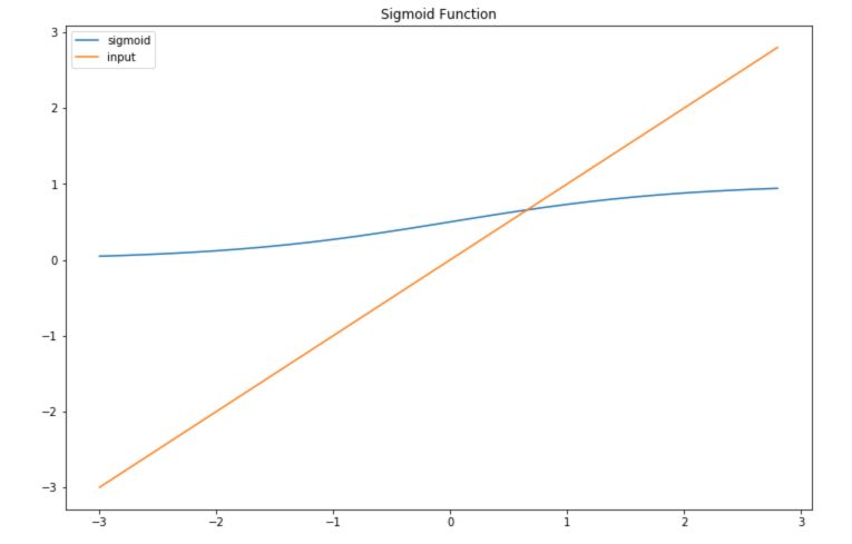
The sigmoid transformation is used to map values between 0 and 1 :
\[Sig(z) = \frac {1} {1 + e^{-z}}\]To understand precisely what this does, let’s implement it in Python :
import numpy as np
import matplotlib.pyplot as plt
import math

def sigmoid(x):
    a = []
    for item in x:
        a.append(1/(1+math.exp(-item)))
    return a
Then, plot if for a range of values of \(X\) :
x = np.arange(-3., 3., 0.2)
sig = sigmoid(x)

plt.figure(figsize=(12,8))
plt.plot(x,sig, label='sigmoid')
plt.plot(x,x, label='input')
plt.title("Sigmoid Function")
plt.legend()
plt.show()
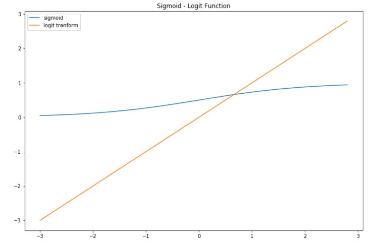
The inverse transform is called the logit transform. It takes values that are in the range 0 to 1 and maps them to a linear form.
def logit(x):
    a = []
    for item in x:
        a.append(math.log(item/(1-item)))
    return a
plt.figure(figsize=(12,8))
plt.plot(x,sig, label='sigmoid')
plt.plot(x,logit(sig), label='logit tranform')
plt.title("Sigmoid - Logit Function")
plt.legend()
plt.show()
The logistic regression model
Partial effect
In the logistic regression model :
\[P(Y=1) = \frac {1} {1 + exp^{-(\beta_0 + \beta_1 X_1 + ... + \beta_p X_p)}}\]How can we interpret the partial effect of \(X_1\) on \(Y\) for example ? Well, the weights in the logistic regression cannot be interpreted as for linear regression. We need to use the logit transform :
\[\log( \frac {P(y=1)} {1-P(y=1)} ) = \log ( \frac {P(y=1)} {P(y=0)} )\] \[= odds = \beta_0 + \beta_1 X_1 + ... + \beta_k X_k\]We define the this ratio as the “odds”. Therefore, to estimate the impact of \(X_j\) increasing by 1 unit, we can compute it this way :
\[\frac {odds_{X_{j+1}}} {odds} = \frac {exp^{\beta_0 + \beta_1 X_1 + ... + \beta_j (X_j + 1) + ... + \beta_k X_k}} {exp^{\beta_0 + \beta_1 X_1 + ... + \beta_j X_j + ... + \beta_k X_k}}\] \[= exp^{\beta_j (X_j + 1) - \beta_j X_j} = exp^{\beta_j}\]A change in \(X_j\) by one unit increases the log odds ratio by the value of the corresponding weight.
Test Hypothesis
To test for a single coefficient, we apply, as previously, a Student test :
\[t_{stat} = \frac {\beta} {\sigma(\beta)}\]For multiple hypotheses, we choose the Likelihood Ratio tests. The coefficients are now normally distributed, so the sum of several coefficients follows a \(X^2\) (Chi-Squared) distribution.
The Likelihood ratio test is implemented in most stats packages in Python, R, and Matlab, and is defined by :
\[LR = 2(L_{ur} - L_r)\]We reject the null hypothesis if \(LR > Crit_{val}\).
Important parameters
In the Logistic Regression, the single most important parameter is the regularization factor. It is essential to choose properly the type of regularization to apply (usually by Cross-Validation).
Implementation in Python
We’ll use Scikit-Learn version of the Logistic Regression, for binary classification purposes. We’ll be using the Breast Cancer database.
# Imports
from sklearn.datasets import load_breast_cancer
from sklearn.model_selection import train_test_split
from sklearn.linear_model import LogisticRegression
from sklearn.metrics import accuracy_score
from sklearn.metrics import f1_score

data = load_breast_cancer()
We then split the data into train and test :
X_train, X_test, y_train, y_test = train_test_split(data['data'], data['target'], test_size = 0.25)
By default, L2-Regularization is implemented. Using L1-Regularization, we achieve :
 lr = LogisticRegression(penalty='l1')
 lr.fit(X_train, y_train)

 y_pred = lr.predict(X_test)
 print(accuracy_score(y_pred, y_test))
 print(f1_score(y_pred, y_test))
 0.958041958041958
 0.9655172413793104
If we move on to L2-Regularization :
 lr = LogisticRegression(penalty='l2', solver='lbfgs')
 lr.fit(X_train, y_train)

 y_pred = lr.predict(X_test)
 print(accuracy_score(y_pred, y_test))
 print(f1_score(y_pred, y_test))
 0.9440559440559441
 0.9540229885057472
We notice the importance of the choice of :
- the solver
- the regularization
We can now illustrate the impact of the tolerance factor C. The larger C is, the less restrictive is the regularization.
 from sklearn.model_selection import GridSearchCV

 parameters = {'C':[0.1, 0.5, 1, 2, 5, 10, 100]}
 lr = LogisticRegression(penalty='l2', max_iter = 5000, solver='lbfgs')

 clf = GridSearchCV(lr, parameters, cv=5)
 clf.fit(X_train, y_train)
We fetch the best parameters using :
clf.best_params_
And find :
{'C': 10}
Using this classifier, we acheive the following results :
 y_pred = clf.predict(X_test)
 print(accuracy_score(y_pred, y_test))
 print(f1_score(y_pred, y_test))
0.958041958041958
0.9655172413793104
We get the same results as with the L1-Penalty, for a rather large value of C. This illustrates well the importance of wisely choosing those parameters, since a 2% accuracy or F1-Score different on a Breast Cancer detection algorithm can make a big difference.
I hope you enjoyed this article. Don’t hesitate to comment if you have any question.
Sources :