Full guide to Linear Regression (2/2)

Before starting this series of articles on Machine Learning, I thought it might be a good idea to go through some Statistical recalls. This first article is an introduction to some more detailed articles on statistics. I will be illustrating some concepts using Python codes.

This is the part 2/2 of our series on Linear Regression.

Random Design Matrix

So far, a hidden hypothesis was set without being explicitly defined: \(X\) should be deterministic. Indeed, we should be able to have full control over how \(X\) is measured. This is what we call a fixed design matrix. Let me quickly introduce an extension of what has been covered so far.

Random Design

In real-life situations, \(X\) is rarely fixed. Indeed, many external components might influence the measures you are currently making. For example, some geological data collected over time could depend on the temperature, the atmospheric pressure or other external factors… And it might not be taken into account.

For this reason, we introduce the random design matrices where : \(X_i = X_i(w)\) is a random variable. The hypothesis on \(\epsilon\) slightly change :

• \[E({\epsilon}_i|X_i) = 0\]
• \[Var({\epsilon}_i|X_i) = {\sigma}^2\]

Consequences

The minimization problem remains the same as previously : \(argmin \sum(Y_i - X \hat{\beta})^2\) .

The difference relies in the associated theoretical results. Recall the Gram matrix that we previously defined : \(G = X^TX\). It should now be written as follows : \(G = E(X^TX)\).

The limit results become : \(\frac {1} {\sqrt{n}} * ({\hat{\sigma}_n - {\sigma}})\) tends as n goes to infinity to \(N(0, E(X^TX)^{-1}{\sigma}^2)\)

Notice that it is now a limit result.

What changes?

What should be remembered from this small article? Well, the direct consequence we face in this case is a change in the confidence interval as the limit distribution is not the same as previously.

Previously, we had :

\({\beta}_{n,k} ± {t}_{1-{\alpha}/2} * \hat{\sigma}_n\), \(t\) being the quantile of the student distribution

This result is constrained to the gaussian hypothesis, which is quite restrictive.

Now that we introduced the random design matrix, the confidence interval becomes :

\({\beta}_{n,k} ± ({\Phi}^{-1})_{1-{\alpha}/2} * \hat{\sigma}_n\) , \({\Phi}^{-1}\) being the quantile of the Normal distribution.

Normal Regression Model

Concept

Recall that in a multi-dimensional linear regression, we have : \(Y = X {\beta}+ {\epsilon}\)

And the following conditions on \({\epsilon}\) :

• \(E({\epsilon}) = 0\) , i.e a white noise condition
• \({\epsilon}_i ∼ iid {\epsilon}\) for all i = 1,…,n, i.e a homoskedasticity condition

Notice also that we never specified any distribution for \({\epsilon}\). This is where the Normal law comes in. This time, we make the hypothesis that : \({\epsilon}_i ∼ iid N(0, {\sigma}^2)\).

Independence implies that :

• \[E({\epsilon}_i|X_i) = E({\epsilon}) = 0\]
• \[Var({\epsilon}_i|X_i) = {\sigma}^2\]

Joint normality is not required in the normal regression model. We simply want to have that the conditional distribution of \(Y\) given \(X\) is normal.

Maximum Likelihood Estimation (MLE)

First, we should observe that the previous condition on the conditional distribution of \(Y\) can be translated into :

\[f(y|X) = \frac {1} {(2{\pi}{\sigma}^2)^{1/2}} e^{- \frac {1} {2{\sigma}^2} (Y - X {\beta})^2}\]

Under the assumption that the observations are independent, the conditional density becomes : \(f(y_1, y_2, ... | x_1, x_2,...) = \prod {f(y_i | x_i)}\)

\[= \prod {\frac {1} {(2{\pi}{\sigma}^2)^{1/2}} e^{- \frac {1} {2{\sigma}^2} (y_i - x_i {\beta})^2} }\] \[= \frac {1} {(2{\pi}{\sigma}^2)^{n/2}} e^{- \frac {1} {2{\sigma}^2} \sum (y_i - x_i {\beta})^2}\] \[= L({\beta}, {\sigma}^2)\]

\(L\) is called the likelihood function. Our aim is to find the Maximum Likelihood Estimation (MLE), i.e the values of \({\beta}\) such that the likelihood function is maximal. A natural interpretation is to identify the values of \({\beta}, {\sigma}^2\) that are the most likely. We can sum up the maximization problem as follows :

\[( \hat{\beta}, \hat{\sigma}^2 ) = {argmax}_{ ({\beta}, {\sigma}^2) } L( {\beta}, {\sigma}^2 )\]

You might have noticed that it is not always simple to work with products in a likelihood function. Therefore, we introduce the log-likelihood function :

\[l({\beta}, {\sigma}^2) = log L({\beta}, {\sigma}^2)\] \[= log f(y_1, y_2, ... | x_1, x_2,...)\] \[= - \frac {n} {2} log (2{\pi}{\sigma}^2) - \frac {1} {2{\sigma}^2} \sum (y_i - x_i {\beta})^2\]

The maximization problem can be re-expressed as :

\[(\hat{\beta}, \hat{\sigma}^2) = {argmax}_{( {\beta}, {\sigma}^2 )} log L({\beta}, {\sigma}^2)\]

First Order conditions

The MLE is usually identified numerically. In our case, we can explore it algebraically, by identifying \(\hat{\beta}, \hat{\sigma}^2\) that jointly solve the First Order Conditions :

\[(1) : \frac {d} {d {\beta}} log L({\beta}, {\sigma}^2) = 0\] \[(2) : \frac {d} {d {\sigma}} log L({\beta}, {\sigma}^2) = 0\]

It can be pretty easily shown that the MLE will give us the same results as the OLS procedure. Indeed, \(\hat{\beta} = {(X^TX)^{-1}X^TY} = \hat{\beta_{OLS}}\)

And :

\[\hat{\sigma}^2 = \frac {1} {n} \sum (y_i - x_i {\beta} )^2 = { \hat{\sigma}_{OLS} }^2\]

The last step is to plug-in the estimators in the initial problem :

\[l({\beta}, {\sigma}^2) = - \frac {n} {2} log (2{\pi}{\sigma}^2) - \frac {1} {2{\sigma}^2} \sum (y_i - x_i {\beta})^2\] \[= - \frac {n} {2} log (2{\pi}\hat{\sigma}^2) - \frac {n} {2}\]

Pseudo Least Squares

Do you remember when we defined the Gram matrix as \(X^TX\) ? To define the OLS estimator, we defined the Gram matrix as invertible. In other words, \(Ker(X) = {0}\) . But what happens when it is not the case?

When does it happen?

It might happen that the Gram matrix is not invertible. But what would that mean? And how does it happen?

• it arises from a non-unique OLS solution
• it typically is the case when the dimension of our design matrix \(X\) is larger than the number of observations itself, e.g collecting a lot of data per patient in a small medical study
• it implies that the pseudo-inverse should be used instead of the inverse of the Gram matrix

Singular Value Decomposition

If we cannot invert the Gram matrix, we are stuck in the algebraic derivation of the OLS model at the following expression :

\[(X^TX){\beta} = X^TY\]

We do not have a unique solution, but a whole set of solutions defined by : \(\hat{\beta} + Ker(X)\).

In order to compute the inverse of \(X^TX\), we need to use the Singular Value Decomposition (SVD). The SVD is a matrix decomposition theorem that states the following :

Any matrix \(X_{(n*n)}\) can be de decomposed as \(X = USV^T\) Where :

• \(U\) is a \((n*n)\) matrix, and \(U^TU = I_n\), contains left singular vectors
• \(S\) is a \((n*p)\) matrix that contains the eigen values of X on the diagonal, and 0s elsewhere.
• \(V\) is a \((p*p)\) matrix, and \(V^TV = I_p\), contains right singular vectors

We can express \(X\) as : \(X = \sum S_iV_i{U_i}^T\)

The whole point of performing an SVD is to define : \(X^+ = \sum {S_i}^{-1}V_i{U_i}^T\). \(X^+\) is called the pseudo-inverse of a matrix. This pseudo-inverse will allow us to compute the pseudo inverse of the Gram matrix :

\[\hat{\beta} = (X^TX)^+ X^TY = (VSU^TUSV^T)^+(VSU^T)Y\] \[= (VS^2V^T)^+(VSU^T)Y = VS^{-2}SU^TY = VS^{-1}U^TY = X^+Y\]

The estimator has now a different form. This means that we can compute again the bias and the variance of this new estimator.

The bias becomes : \(E(\hat{\beta}) - {\beta} = X^+E(Y) - {\beta} = X^+(X{\beta}) - {\beta}\) \(= (X^+X - I_p){\beta}\) where \(X^+X\). The estimator will be biaised, except if \(X^+X - I_p = 0\) which means \(Ker(X) = {0}\).

The variance becomes : \(Var(\hat{\beta}_n) = (X^TX)^+{\sigma}^2\) \(= (VSU^TUSV^T)^+{\sigma}^2 = (VS^{-2}V^T){\sigma}^2\) \(= \sum \frac {({\sigma}_i)^2} {(S_i)^2} V_i {V_i}^T\)

Transformations

Let’s get back to the simple problem in which we wanted to assess the demand for ice cream depending on the outside temperature. The model we built looked like this :

\[y_i = \beta_0 + \beta_1 * x_i + u_i\]

where :

• \(y_i\) is the icecream demand on a given day
• \(\beta_0\) a constant parameter
• \(\beta_1\) the parameter that assesses the impact of temperature on icecream demand
• \(x_i\) the average temparature for a given day
• \(u_i\) the residuals

However, the assumption that the model is purely linear is strong, that is pretty much never met in practice. We can apply some transformations to the model to make it more flexible.

1. Log

\[log(y_i) = \beta_0 + \beta_1 * x_i + u_i\]

This also means that 1% change of \(y_i\) : \(\delta_{y_i}\) is equal to \(100 * \beta_1 * \delta_{x_i}\) .

2. Log-Log

\[log(y_i) = \beta_0 + \beta_1 * log(x_i) + u_i\]

3. Square Root

\[y_i = \beta_0 + \beta_1 * \sqrt {x_i} + u_i\]

4. Quadratic

\[y_i = \beta_0 + \beta_1 * {X_1}_i + \beta_2 * {X_{2i}}^2 + u_i\]

This implies that :

\[\frac { \delta_{ {X_1}_i } } { \delta_{ {X_2}_i } } = \beta_1 + 2 * \beta_2 * {X_2}_i\]

5. Non-linear

\[y_i = \frac {1} {\beta_0 + \beta_1 * {x}_i } + u_i\]

This is a simple example of a non-linear transform.

Boolean and Categorical Variables

Up to now, we mostly considered cases in which the variables were continuous (temperature for example). But the variety of data you might deal with might include categorical or boolean variables!

I. Binary Variables

Let’s get back to our icecream demand forecasting problem :

\[y_i = \beta_0 + \beta_1 * x_i + u_i\]

where :

• \(y_i\) is the icecream demand on a given day
• \(\beta_0\) a constant parameter
• \(\beta_1\) the parameter that assesses the impact of temperature on icecream demand
• \(x_i\) the average temparature for a given day
• \(u_i\) the residuals

A binary variable that might be interesting to predict icecream’s consumption is the fact that there is public holiday on the day considered or not :

\[y_i = \beta_0 + \beta_1 * {X_1}_i + \beta_2 * {X_2}_i + u_i\]

where :

• \({X_2}_i = 1\) is there is public holiday this day
• \({X_2}_i = 0\) otherwise

Therefore, we can see \(\beta_2\) as :

\[\beta_2 = E (y_i \mid holiday, {X_1}_i) - E (y_i \mid no-holiday, {X_1}_i )\]

Public holiday has an impact on icecream demand if \(\beta_2\) is significantly different from 0. This can be seen as a classical hypothesis testing :

• Null hypothesis \(H_0 : \beta_2 = 0\)
• and \(H_0 : \beta_2 ≠ 0\)

II. Categorical Variables

We might also have more than 2 categories. For example, regarding our public holiday variable, we’ll now be interested in which state/region of France is on a public holiday (there are 3 overall, to avoid have everybody sharing the same week of holidays).

\[y_i = \beta_0 + \beta_1 * {X_1}_i + \beta_2 * {X_2}_i + \beta_3 * {X_3}_i + \beta_4 * {X_4}_i + u_i\]

where :

• \({X_2}_i = 1\) is zone A is on holiday
• \({X_3}_i = 1\) is zone B is on holiday
• \({X_4}_i = 1\) is zone C is on holiday

The reference case we implicitly consider here is the case in which there is no public holiday. The three terms are here to evaluate a difference with the reference case.

We can run individual or joint tests on the different coefficients of the regression.

III. Interaction variable

The intuition behind the interaction variable is quite simple. Suppose we want to test the effect of temperature on consumption if zone A is on holiday.

The problem can be formulated as follows :

\[y_i = \beta_0 + \beta_1 * {X_1}_i + \beta_2 * {X_2}_i + \theta_2 * {X_2}_i * {X_1}_i + \beta_3 * {X_3}_i + \beta_4 * {X_4}_i + u_i\]

Here, \(\theta_2\) measures the effect of temperature on icecream consumption when zone A is on holiday.

We can run student tests on \(\theta_2\) directly.

We can now enrich our model and add several interaction terms :

\[y_i = \beta_0 + \beta_1 * {X_1}_i + \beta_2 * {X_2}_i + \theta_2 * {X_2}_i * {X_1}_i + \beta_3 * {X_3}_i + \theta_3 * {X_3}_i * {X_1}_i + \beta_4 * {X_4}_i + \theta_4 * {X_4}_i * {X_1}_i + u_i\]

If we want to test the difference between the groups, we should make a Fisher test with a null hypothesis \(H_0 : \theta_2 = 0, \theta_3 = 0, \theta_4 = 0\).

Dealing with heteroscedasticity

Heteroscedasticity might be an issue when conducting hypothesis tests. How can we define heteroscedasticity? How can we detect it? How can we overcome this issue?

I. What is heteroscedasticity?

Heteroscedasticity (or heteroskedasticity) refers to the case in which the variability is unequal across the range of values.

Recall that in the linear regression framework : \(y = \beta_0 + \beta_1 X_1 + ... + \beta_k X_k + u\). The fundamental hypothesis is that : \(E (u \mid X_1, X_2, ..., X_k) = 0\). Under this hypothesis, the OLS estimator is the Best Linear Unbiaised Estimator (BLUE).

By normality hypothesis, under homoscedasticity, \(u \sim N(0, \sigma^2)\) and \(Var (u \mid X_1, ... X_k) = \sigma^2\).

For example, if we try to predict the income in terms of the age of a person :

• in case of homoscedasticity, the variance is constant over the age of the person, i.e
• in case of heteroscedasticity, the variance is increasing over the age of the person

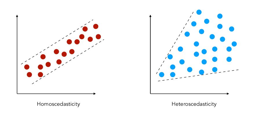
Under heteroscedasticity, \(Var (u_i \mid X_i) = {\sigma_i}^2\).

II. Transform the variables in log

In most cases, to control for heteroscedasticity, there is an easy trick: transform the variables in log.

\[log(y) = \beta_0 + \beta_1 X_1 + ... + \beta_k X_k + u\]

Most of the time, this will do the trick!

For example, in Matlab :

y = log(hprice1(:,1));
[n,k] = size(hprice1);

X = [ones(n,1), hprice1(:,[3,4,5])]
beta = inv(X'*X)*X'*y

III. Robust inference to heteroscedasticity

Concept

*Idea *: Build a standard error robust to any kind of heteroscedasticity.

The estimators take the following form :

\[\hat{\beta_1} = \beta_1 + \frac {\sum_i (X_i - \bar{X})^2 \hat{u_i}^2} { \sum_i (X_i - \bar{X})^2}\]

This estimator is robust to any kind of heteroscedasticity. The variance of the estimator is defined by :

\[Var( \hat{\beta_1} ) = \frac { \sum_i ( X_i - \bar{X})^2 {\sigma_i}^2 } { { SSR_x }^2 }\]

This requires \(\beta_1\) to be known and \(u_i\) too. We can define \(\hat{u_i}\) the residual of the estimation. Using White’s formula:

\(\frac { \sum_i (X_i - \bar{X})^2 \hat{u_i}^2 } { { SSR_x }^2 }\) is robust to any kind of heteroscedasticity.

Therefore, if \(r_{ij}\) is the residual of the regression of \(X_{j}\) on the other independant variables, we have :

\[\hat{Var}( \hat{\beta_j} ) = \frac {\sum_i \hat{r_{ij}}^2 \hat{u_i}^2 } { {SSR_j}^2 }\]

It is sufficient to modify the reference standard error during further tests.

Detect heteroscedasticity

How can we detect heteroscedasticity ? A simple test hypothesis can be used :

\[H_0 : Var(u \mid X_1, ..., X_k) = \sigma^2\]

IV. Linear form residuals

The residuals in case of heteroscedasticity might depend on :

• time, with an index \(i\), as we have seen up to now
• other features

In the second case, the residuals should have the following form :

\[u^2 = \delta_0 + \delta_1 X_1 + ... + \delta_k X_k + V\]

We can test the hypothesis \(H_0 : \delta_1 = \delta_2 = ... = \delta_k = 0\)

V. Heteroscedasticity with a constant shift

This time, the hypothesis is the following :

\[Var(u \mid x_i) = \sigma^2 h(x_i)\]

Therefore, we might need to modify the residuals :

\[E( ( \frac {u_i} {\sqrt{h_i} } )^2 ) = \frac {E({u_i}^2)} {h_i} = \frac { \sigma^2 h_i} {h_i} = \sigma^2\]

Now, let’s use the transformed model to fit our regression :

\[\frac {y_i} {\sqrt{h_i} } = \frac {\beta_0} {\sqrt{h_i} } + \beta_1 \frac { X_{i1} } { \sqrt{h_i} } + ... + \beta_k \frac { X_{ik} } { \sqrt{h_i} } + \frac {u_i} { \sqrt{h_i} }\]

We obtain a weighted least squares problem :

\[\frac {\sum_i (y_i - b_0 - b_1 X_{i1} - ... - b_k X_{ik})^2 } {h_i}\]

In practice, it is hard to find those weights. For this reason, we usually apply what we call generalized least squares (GLS).

Generalized Least Squares

In the previous sections, we highlighted the need for models and estimators that handle heteroscedasticity. We’ll introduce Generalized Least Squares, a more general framework.

Recall that in the OLS framework, the Best Linear Unbiaised Estimator was defined by :

\[b = (X' X)^{-1} X' Y = \beta + (X'X)^{-1}X' \epsilon\]

We have seen previously that under heteroscedasticity, this estimator was no longer the best. It remained, however, a Linear Unbiased Estimator.

Suppose that we know \(\Omega\) the covariance of the errors such that it can be split the following way by Cholesky decomposition: \(\Omega^{-1} = P'P\), \(P\) a triangular matrix.

In this case, we can build the GLS estimator by scaling the initial regression problem :

\[Py = PX \beta + P \epsilon\]

We can define new shifted variables :

\[Y^{*} = X^{*} \beta + \epsilon^{*}\]

The resulting estimator is therefore modified too :

\[\hat{\beta} = (X^{'*} X^{*})^{-1} X^{'*} Y^{*} = (X'P'PX)^{-1}X'P'Py = (X' \Omega^{-1} X)^{-1} X' \Omega^{-1} y\]

The variance of the estimator becomes :

\[Var( \hat{\beta} \mid X*) = \sigma^2(X'*X'*)^{-1} = \sigma^2(X' \Omega^{-1} X)^{-1}\]

1. Weighted Least Squares

The Weighted Least Squares is a special case of the GLS framework.

Under heteroscedasticity, we might face : \(Var( \epsilon_i \mid X_i) = {\sigma_i}^2 = \sigma^2 w_i\)

In such case, we can specify \(\Omega^{-1}\), which has diagnoal elements of the type \(\frac {1} {w_i}\)

If we replace the next value of \(\Omega\) in the GLS estimator :

\[\hat{\beta} = ( \sum_i w_i X_i X_i' )^{-1} ( \sum_i w_i X_i y_i)\]

The estimator is consistent whatever the weights being used.

2. Feasible Least Squares

Usually, we don’t know the covariance of the errors, but it usually depends on some parameters that can be estimated. This is the main idea behind Feasible Least Squares.

\[\hat{ \omega} = \Omega ( \hat{ \theta} )\]

We can use this estimator in the estimator’s formula :

\[\hat {\hat { \beta } } = (X' \hat{ \Omega^{-1}} X)^{-1} X' \hat{\Omega^{-1}} Y\]

The Github repository of this article can be found here.