
Before starting this series of articles on Machine Learning, I thought it might be a good idea to go through some Statistical recalls. This first article is an introduction to some more detailed articles on statistics. I will be illustrating some concepts using Python codes.
Linear Regression in 1 dimension
Framework
The most basic statistical foundation of machine learning models is the following : \(Y_i = f(X_i) + {\epsilon}\) . This simple equation states the following :
- we suppose we have \(n\) observations of a dataset, and we pick on \(i^{th}\)
- \(Y_i\) is the output of this observation called the target
- \(X_i\) is called a feature and is an independent variable we observe
- \(f\) is the real model that states the link between the features and the output
- \({\epsilon}\) is the noise of the model. The data we observe usually do not stand on a straight line, because there are variations of the measure in real life.
The framework we consider here is pretty simple. We only have one feature per observation. In real life, we do usually have several features per observation. An example of this might be the following: you work as a data scientist in an insurance company. You would typically have several pieces of information on each customer: name, address, age, family, car, salary…
Statistical motivation
Suppose that we have \(n\) observations, and for each observation i, we have one feature \(X_{i}\).
Our role is to identify the link between \(Yi\) and \(X_{i}\) in order to be able to predict \(Y_{n+1}\) . To build our prediction, we need to identify :
- a model, which is the link between \(Y_i\) and the features, represented here by the function \(f\) in : \(Y_i = f(X_i) + {\epsilon}\) . In real life, this model \(f\) is unknown in real life and is estimated by : \(\hat{Y}_i = \hat{f}(X_i)\) where the hat describes an estimation. We try to estimate \(\hat{f}\) that corresponds to real life \(f\).
- we also need to identify parameters, which will help our prediction to get as close as possible to real datas. The parameters are usually set in order to minimize the distance between our model and the datas, i.e they are set so that the derivative of a loss function (for example : \(\sum(\hat{Y_i} - Y_i)^2 )\) is equal to 0.
The true model and the true parameters in real life are unknown. For this reason, we make a selection among several models (linear or non-linear). The model selection is usually based on an exploratory data analysis. An article will further develop this question.
From now on, we will focus on the most basic model called the unidimensional linear regression. This model states that there is a linear link between the features and the dependent variable.
The true model we expect is the following : \(Y_i = {\beta}_0 + {\beta}_1{X}_{i} + {\epsilon}_i\)
- \({\beta}_0\) is called the intercept, it is a constant term
- \({\beta}_1\) is the coefficient associated with \(X_i\) . It describes the weight of \(X_i\) on the final output.
- \({\epsilon}_i\) is called the residual. It is a white noise term that explains the variability in real life datas.
The hypothesis on \({\epsilon}\) are :
- \(E({\epsilon}) = 0\) , i.e a white noise condition
- \({\epsilon}_i ∼ iid {\epsilon}\) for all i = 1,…,n, i.e a homoskedasticity condition
However, the true parameters remain unknown as these are the ones we expect to estimate. Therefore, the model we estimate is the following : \(\hat{Y}_i = \hat{\beta}_0 + \hat{\beta}_1{X}_{i}\) .
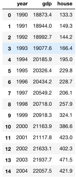
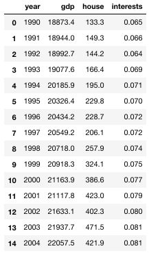
A classic example would be to try to predict the average housing market price in the economy based on the GDP for example. We would expect pretty much a linear relationship between both. You can find the file I will be using here
import pandas as pd
import numpy as np
import matplotlib.pyplot as plt
import sklearn.linear_model as lm
import math
from scipy import stats

df = pd.read_csv('housing.txt', sep=" ")
df
#Scatter plot
plt.figure(figsize=(7,5))
plt.scatter(df['gdp'], df['house'])

#On ajoute les titres des axes
plt.xlabel("Gross Domestic Product)", fontsize = 12)
plt.ylabel("Housing price", fontsize = 12)
plt.title("Relation between GDP and Average housing prices")

plt.show()
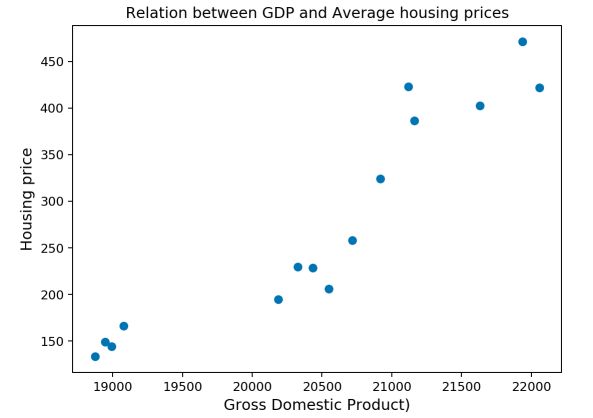
Our intuition was right. The relationship looks linear between the GDP and the average housing price. How do we move on from here?
Parameter estimate
Now that we know the relationship looks linear, the next step is to estimate the coefficients \(\hat{\beta}_0 , \hat{\beta}_1\) in order to draw a line that fits our datas. In the linear regression, estimating the parameter means identifying the Betas : \(\hat{\beta}_0 , \hat{\beta}_1\) so that they minimize the distance with the real datas :
\(argmin \sum(Y_i - \hat{\beta}_0 - \hat{\beta}_1{X}_{i})^2\) .
This approach is known as the Ordinary Least Squares (OLS). We minimize the square of the distance between each data point and our estimate. Why the square? Because the derivative is easier to find, and we take both positive and negative deviations into account.
The solution of the OLS problem in 1 dimension is the following : \(\hat{\beta}_1 = \frac{\sum(X_i – \bar{X}) (Y_i – \bar{Y})} {\sum(X_i – \bar{X})^2}\) \(\hat{\beta}_0 = \bar{Y} – \hat{\beta}_1 \bar{X}\)
We can compute those results in Python :
# Slope Beta 1 :
x = df['gdp']
x_bar = mean(df['gdp'])
y = df['house']
y_bar = mean(df['house'])

beta1 = ((x - x_bar)*(y-y_bar)).sum() / ((x-x_bar)**2).sum()
print("Beta_1 coefficient estimate : " + str(round(beta1,4)))
0.1012
beta0 = y_bar - beta1 * x_bar
print("Beta_0 coefficient estimate : " + str(round(beta0,4)))
-1794.0861
We can plot the estimated linear regression to assess whether it looks good or not :
#Scatter plot
plt.figure(figsize=(7,5))
plt.scatter(df['gdp'], df['house'])
plt.plot(df['gdp'], beta1 * df['gdp'] + beta0, c='r')
#On ajoute les titres des axes
plt.xlabel("Gross Domestic Product)", fontsize = 12)
plt.ylabel("Housing price", fontsize = 12)
plt.title("Relation between GDP and Average housing prices")

plt.show()
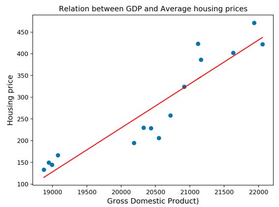
It looks great ! There is a pretty efficient way to do this using Scikit Learn built-in functions.
x_1 = df[['gdp']]
skl_linmod = lm.LinearRegression(fit_intercept = True).fit(x_1,y)

beta1_sk = skl_linmod.coef_[0]
beta0_sk = skl_linmod.intercept_
This will head the same results. Alright, so far we are satisfied by how our estimate looks like. But how do we assess how good our estimate is?
Assess the accuracy of the estimate using R2
A common metric used to assess the overall fit of our model is the \(R^2\) metric (pronounced R squared). The \(R^2\) measures the percentage of the variance of the datas we manage to explain with our model :
\[{R^2} = \frac{\sum(Y_i – \hat{Y})^2} {\sum(Y_i – \bar{Y})^2}\]r_carre = 1 - (((y-(beta0 + beta1 * x))**2).sum())/((y-y_bar)**2).sum()
0.861
The \(R^2\) takes values between 0 and 1. The closer we are to 1, the more variance we tend to explain. However, adding variables will always make the \(R^2\) increase, even if the variable we added is not related to the output at all. I do invite you to check the adjusted - \(R^2\) if you would like to know more about how to handle this issue.
Are coefficients significant?
Alright, we have now fitted our regression line and estimated the goodness of the fit. But all the variables included in the model might not be worth including? What if for example \({\beta}_1\) is not significantly different from 0 ?
Both parameters \({\beta}_0, {\beta}_1\)can be described by three metrics :
- an expectation
- a bias
- a variance
The expectation of the parameter corresponds… to its expected value. Nothing really new here : \(E(\hat{\beta}_j)\)
The bias corresponds to how far we are from the actual value. It is given by : \(E(\hat{\beta}_j) - {\beta}_j\) . The true bias is typically unknown, as we try to estimate \({\beta}_j\) . If the bias is 0, we say that the estimator is unbiased.
The variance defines the stability of our estimator regarding the observations. Indeed, the features might be highly spread, which would mean a pretty big variance.
It can be shown that the variance of \({\beta}_1\) is given by : \(\hat{\sigma}{_\hat{\beta_1}} = \frac{\hat{\sigma}} {\sqrt{\sum(X_i – \bar{X})^2}}\)
And the one of \({\beta}_0\) by : \(\hat{\sigma}{_\hat{\beta_0}} = \hat{\sigma} \sqrt{\frac{1} {n} + \frac{\sum(X_i)^2} {\sum(X_i – \bar{X})^2}}\)
Where the estimated variance \(\hat{\sigma}\) is defined by : \(\hat{\sigma} = \sqrt\frac{\sum(Y_i – \hat{Y}_i)^2} {n – p-1}\) . This is an unbiaised estimator of the variance.
Now, we do have all the elements required to compute the standard errors of our parameters :
sigma2 = math.sqrt(np.var(y))
sigma_beta1 = math.sqrt(sigma2 / ((x-x_bar)**2).sum())
0.00264
sigma_beta0 = math.sqrt(sigma2 * (1/len(y) + (x_bar**2)/((x-x_bar)**2).sum()))
54.09148485682019
Graphically, biais and variance can be represented this way :
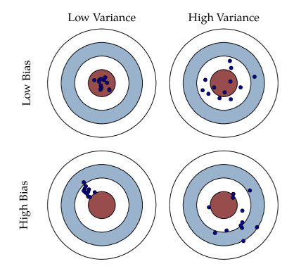
Why are we spending time on those metrics? Those metrics allow us to compute what we call test hypothesis.
Test Hypothesis
For each parameter, we want to test whether the parameter in question has a real impact on the output or not, to avoid adding dimensions that bring no significant information. In the linear regression : \(\hat{Y}_i = \hat{\beta}_0 + \hat{\beta}_1{X}_{i}\) , it would mean testing whether the Betas are significantly different from 0 or not.
To do so, we proceed to a statistical test. If our aim is the state if the parameter is significantly different from 0, we are doing a test with : \(H_0\) the null hypothesis : \({\beta}_j = 0\) and \(H_1\) the alternative hypothesis : \({\beta}_j ≠ 0\) .
Some further theory is needed here : Recall the Central Limit Theorem. \(\sqrt{n} \frac{\bar{Y}_n - {\mu}} {\sigma}\) converges to \(∼ {N(0,1)}\) as n tends to infinity if \({\sigma}\) is knowm.
In case \({\sigma}\) is unknown, Slutsky’s Lemma states that \(\sqrt{n} \frac{\bar{Y}_n - {\mu}} {\hat{\sigma}}\) converges to \(∼ {N(0,1)}\) if \({\hat{\sigma}}\) converges to \({\sigma}\) .
Most of the time, \({\sigma}\) is unknown. From this point, it can be shown that : \(\hat{T}_j = \frac{\hat{\beta}_j - 0} {\hat{\sigma}_j} ∼ {\tau}_{n-p-1}\) where \({\tau}_{n-p-1}\) and \(n-p-1\) is the degrees of freedom (p is the dimension, equal to 1 here).
This metric is called the T-Stat, and it allows us to perform a hypothesis test. The 0 in the numerator can be replaced by any value we would like to test actually.
How to interpret the T-Stat?
The T-Stat should be compared with the Critical Value. The critical value is the quantile of the corresponding Student distribution at a given level of \({\alpha}\). If a coefficient is significant at a level \({\alpha}\) , this means that the T-Stat is above or under the quantiles of the Student Distribution.
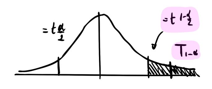
Another interpretation is that the probability that the coefficient estimate is not in the interval \([- {t}_{1-{\alpha}/2}; + {t}_{1-{\alpha}/2} ]\) is smaller than \({\alpha}\) . This probability is called the p-value and is defined by : \(p_{value} = Pr( |\hat{T}_j| > |{t}_{1-{\alpha}/2}|)\)
Thus, in a null test, we do reject \(H_0\) at a level \({\alpha}\) (typically 5%) if and only if the p-value is smaller than \({\alpha}\) , i.e the probability to be in the interval around 0 is really small.
from scipy import stats

t_test = beta1 / sigma_beta1
print("The T-Stat is : " + str(round(t_test,4)))

p = (1 - stats.t.cdf(abs(t_test), len(df)-2)) * 2
print("The p-value is : " + str(round(p,10)))
The T_stat is : 38.3198
The p-value is : 0.0
In our example, the T-Stat is pretty big, bigger than the corresponding quantile at 5% of the Student distribution, and the p-value is by far smaller than 5%. Therefore, we reject the null hypothesis : \(H_0 : {\beta}_1 = 0\) and we conclude that the parameter \({\beta}_1\) is not null.
Confidence Interval for the parameters
Finally, a notion one should get familiar with is the notion of confidence interval. Using the CLT, one can set a confidence interval around an estimate of a parameter.
The lower bound and the upper bound are determined by the critical value of the student distribution at a level \({\alpha}\), and by the standard deviation of the parameter. \({\beta}_1 ± {t}_{1-{\alpha}/2} * \hat{\sigma}_{\hat{\beta_1}}\)
t_crit = stats.t.ppf(0.975,df=len(y) - 2)

c0 = beta1 - t_crit * sigma_beta1
c1 = beta1 + t_crit * sigma_beta1
0.0954, 0.1068
The same process can be done for the parameter \({\beta}_0\)
Type I and Type II risks
Rejecting or not a hypothesis comes at a cost: one could misclassify a parameter.
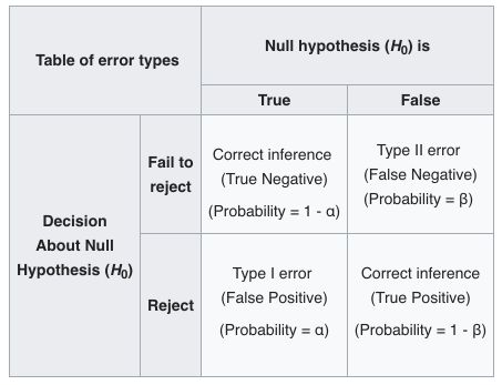
The Type I risk is the probability to reject \(H_0\) whereas it is true. The Type II risk is the probability to not reject \(H_0\) whereas it is false.
The Level of a test is 1 - Type I risk, and represents the probability to not-reject \(H_0\) when \(H_0\) is true.
Wikipedia summarizes this concept pretty well :
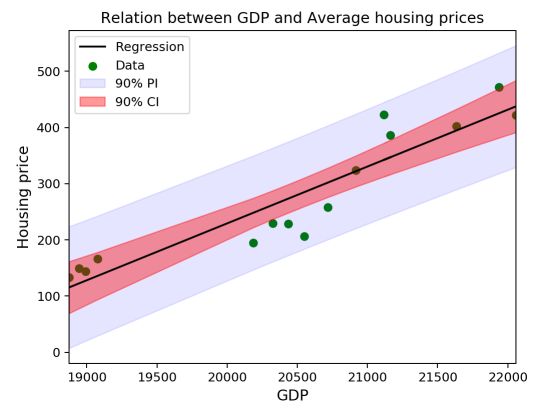
Confidence Interval for the model
We can define two types of confidence intervals for the model. The first one is the estimation error confidence interval. We need to take into account the error around \({\beta_1}\) and around \({\beta_0}\) :
\[CI(x) = \hat\beta_0 + \hat\beta_1 x \, \pm \, t_{1 - \frac{\alpha}{2}}^{(n-2)} \, \hat\sigma\sqrt{\frac{1}{n} + \frac{(x - \overline{x})^2}{\sum_{i=1}^n(x_i - \overline{x})^2}}\]Moreover, the prediction risk is different. The prediction risk corresponds to the risk associated with the extension of our model onto a new prediction : \(Y_{new} = \hat{Y} + {\epsilon} ; {\epsilon} ∼ N(0,{\sigma}^2)\) . We have a new source of volatility : \({\epsilon}\) . And this leads to a modified confidence interval :
\[PI(x) = \hat\beta_0 + \hat\beta_1 x \, \pm \, t_{1 - \frac{\alpha}{2}}^{(n-2)} \, \hat\sigma\sqrt{1 + \frac{1}{n} + \frac{(x - \overline{x})^2}{\sum_{i=1}^n(x_i - \overline{x})^2}}\]These two confidence intervals can be plotted on the previous graph :
plt.figure()
y = df['house']
plt.scatter(df['gdp'], df['house'], label = "Data", color = "green")
plt.plot(df['gdp'], beta0 + beta1 * x, label = "Regression", color = "black")

plt.fill_between(df['gdp'], beta0 + beta1 * x - t_crit * np.sqrt(sigma2 * (1 + 1/len(y) + (x - x_bar)**2/((x-x_bar)**2).sum())), beta0 + beta1 * x + t_crit * np.sqrt(sigma2 * (1 + 1/len(y) + (x - x_bar)**2/((x-x_bar)**2).sum())), color = 'blue', alpha = 0.1, label = '90% PI')
plt.fill_between(df['gdp'], beta0 + beta1 * x - t_crit * np.sqrt(sigma2 * (1/len(y) + (x - x_bar)**2/((x-x_bar)**2).sum())), beta0 + beta1 * x + t_crit * np.sqrt(sigma2 * (1/len(y) + (x - x_bar)**2/((x-x_bar)**2).sum())), color = 'red', alpha = 0.4, label = '90% CI')

plt.legend()
plt.xlabel("GDP", fontsize = 12)
plt.ylabel("Housing price", fontsize = 12)
plt.title("Relation between GDP and Average housing prices")
plt.xlim(min(x), max(x))
plt.show()
Linear Regression in 2 dimensions
So far, we have covered the unidimensional linear regression framework. But as you might expect, this is only a simple version of the linear regression model. Back to our housing price problem. So far, we only included the GPD variable. But as you may know, interest rates are also major leverage on the housing market.
Framework
The more general framework can be described as : \(Y = X {\beta}+ {\epsilon}\) . Notice that we are now in matrix form. Indeed :
- we suppose we have n observations of a dataset and p features per observation
- \(Y\) is the output of this observation
- \({\beta}\) is the column vector that contains the true parameters
- \(X\) is now a matrix of dimension (nxp)
Otherwise, the conditions on \({\epsilon}\) remain the same.
- \(E({\epsilon}) = 0\) , i.e a white noise condition
- \({\epsilon}_i ∼ iid {\epsilon}\) for all i = 1,…,n, i.e a homoskedasticity condition
In the 2 dimension problem introduced above to predict the housing prices, our task is now to estimate the following model : \(\hat{Y}_i = \hat{\beta}_0 + \hat{\beta}_1{X}_{1i} + \hat{\beta}_2{X}_{2i}\)
The dataset I’m using can be found here.
import pandas as pd
import numpy as np
import math

df = pd.read_csv('https://maelfabien.github.io/myblog/files/housing.txt', sep=" ")
df
fig, axs = plt.subplots(2, figsize=(8,8))

axs[0].scatter(df['gdp'], df['house'])
axs[1].scatter(df['interests'], df['house'], c='r')

axs[0].set_xlabel("Gross Domestic Product", fontsize = 12)
axs[0].set_ylabel("Housing Price", fontsize = 12)
axs[0].set_title("Relation between GDP and Average Housing Prices")

axs[1].set_xlabel("Interest rates", fontsize = 12)
axs[1].set_ylabel("Housing Price", fontsize = 12)
axs[1].set_title("Relation between interest rates and Average Housing Prices")

plt.tight_layout()

plt.show()
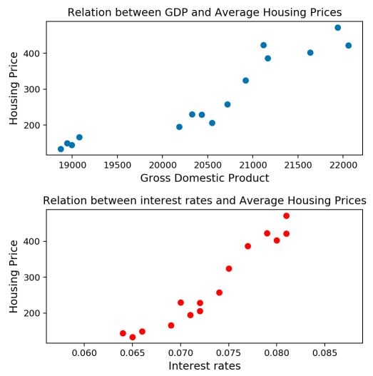
The linear relationship with the interest rate seems to hold again! Let’s dive into the model.
OLS estimate
Recall that to estimate the parameters, we want to minimize the sum of squared residuals. In the higher dimension, the minimization problem is :
\(argmin \sum(Y_i - X \hat{\beta})^2\) .
In our specific example, \(argmin \sum(Y_i - \hat{\beta}_0 - \hat{\beta}_1 {X}_{1i} - \hat{\beta}_2 {X}_{2i})^2\)
The general solution to OLS is : \(\hat{\beta} = {(X^TX)^{-1}X^TY}\) . Simply remember that this solution can only be derived if the Gram matrix defined by \(X^TX\) is invertible. Equivalently, \(Ker(X) = {0}\) . This condition guarantees the uniqueness of the OLS estimator.
x = np.hstack([np.ones(shape=(len(y), 1)), df[['gdp', 'interests']]]).astype(float)
xt = x.transpose()
X_gram = x
gram = np.matmul(xt, x)
i_gram = inv(gram)
We can use the Gram matrix to compute the estimator \(\hat{\beta}\) :
Beta = np.matmul(inv(gram), np.matmul(xt,y))

#Display coefficients Beta0, Beta1 and Beta2
print("Estimator of Beta0 : " + str(round(Beta[0],4)))
print("Estimator of Beta1 : " + str(round(Beta[1],4)))
print("Estimator of Beta2 : " + str(round(Beta[2],4)))
Estimator of Beta0 : -1114.2614
Estimator of Beta1 : -0.0079
Estimator of Beta2 : 21252.7946
We will discuss cases in which this condition is not met in the next article.
Orthogonal projection
Note that \(\hat{Y} = X \hat{\beta} = X(X^TX)^{-1}X^TY = H_XY\) where \(H_X = X(X^TX)^{-1}X^T\) . We say that \(H_X\) is an orthogonal projector since it meets two conditions :
- \(H_X\) is symmetrical : \({H_X}^T = H_X\)
- \(H_X\) is idempotent : \({H_X}^2 = H_X\)
Graphically, this projection states that we project \(\hat{Y}\) onto the hyperplane formed by the columns of X.
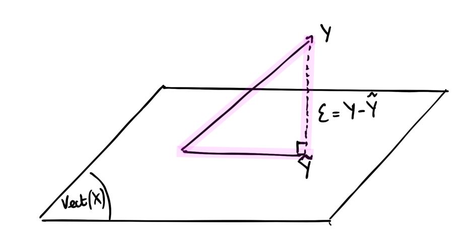
This allows us to redefine the vectors of residuals : \({\epsilon} = Y - \hat{Y} = (I - H_X)Y\) where \(I\) is the identity matrix.
\((I - H_X)\) is an orthogonal projector on the orthogonal of \(Vect(X)\) .
Bias and Variance of the parameters
Notice that \(\hat{\beta} - {\beta} = (X^TX)^{-1}X^TY - (X^TX)^{-1}X^TX{\beta} = (X^TX)^{-1}X^T{\epsilon}\)
The bias of the parameter is defined by : \(E(\hat{\beta}) - {\beta} = E(\hat{\beta} - {\beta}) = E((X^TX)^{-1}X^T{\epsilon}) = (X^TX)^{-1}X^TE({\epsilon}) = 0\) . The estimate \(\hat{\beta}\) of the parameter \({\beta}\) is unbiaised.
The variance of the parameter is given by : \(Cov(\hat{\beta}) = (X^TX)^{-1}X^TCov({\epsilon})X(X^TX)^{-1} = (X^TX)^{-1}{\sigma}^2\) . Therefore, for each \({\beta}_j\) : \(\hat{\sigma}^2_j = \hat{\sigma}^2{(X^tX)^{-1}_{j,j}}\)
#Standard errors of the coefficients
sigma = math.sqrt(((y - Beta[0] - Beta[1] * xt[1] - Beta[2]*xt[2])**2).sum()/(len(y)-3))
sigma2 = sigma ** 2

se_beta0 = math.sqrt(sigma2 * inv(gram)[0,0])
se_beta1 = math.sqrt(sigma2 * inv(gram)[1,1])
se_beta2 = math.sqrt(sigma2 * inv(gram)[2,2])

print("Estimator of the standard error of Beta0 : " + str(round(se_beta0,3)))
print("Estimator of the standard error of Beta1 : " + str(round(se_beta1,3)))
print("Estimator of the standard error of Beta2 : " + str(round(se_beta2,3)))
Estimator of the standard error of Beta0 : 261.185
Estimator of the standard error of Beta1 : 0.033
Estimator of the standard error of Beta2 : 6192.519
The significance of each variable is assessed using an hypothesis test : \(\hat{T}_j = \frac{\hat{\beta}_j} {\hat{\sigma}_j}\)
#Student t-stats
t0 = Beta[0]/se_beta0
t1 = Beta[1]/se_beta1
t2 = Beta[2]/se_beta2
print("T-Stat Beta0 : " + str(round(t0,3)))
print("T-Stat Beta1 : " + str(round(t1,3)))
print("T-Stat Beta2 : " + str(round(t2,3)))
T-Stat Beta0 : -4.266
T-Stat Beta1 : -0.242
T-Stat Beta2 : 3.432
Something pretty interesting happens here: by adding a new variable to the model, the coefficient of \({\beta}_1\) quite logically changed but became non-significant. We do expect \({\beta}_2\) to explain the model way better now.
The Quadratic Risk is : \(E[(\hat{\beta} - {\beta})^2] = {\sigma}^2 \sum{\lambda}_k^{-1}\) where \({\lambda}_k\) are the eigenvalues of the Gram matrix.
The prediction risk is : \(E[(\hat{Y} - Y)^2] = {\sigma}^2 (p+1)\)
The Github repository of this article can be found here.