
In this article, we’ll introduce the key concepts related to time series.
We’ll be using the same data set as in the previous article: Open Power System Data (OPSD) for Germany. The data can be downloaded here
Start by importing the following packages :
### General import
import numpy as np
import pandas as pd
import matplotlib.pyplot as plt
import seaborn as sns
from sklearn import preprocessing
import statsmodels.api as sm

### Time Series
from statsmodels.tsa.ar_model import AR
from sklearn.metrics import mean_squared_error
from pandas.tools.plotting import autocorrelation_plot
from statsmodels.tsa.arima_model import ARIMA
from statsmodels.tsa.seasonal import seasonal_decompose
from statsmodels.tsa.stattools import adfuller
#from statsmodels.tsa.sarimax_model import SARIMAX

### LSTM Time Series
from keras.models import Sequential
from keras.layers import Dense
from keras.layers import LSTM
from keras.layers import Dropout
from sklearn.preprocessing import MinMaxScaler
Then, load the data :
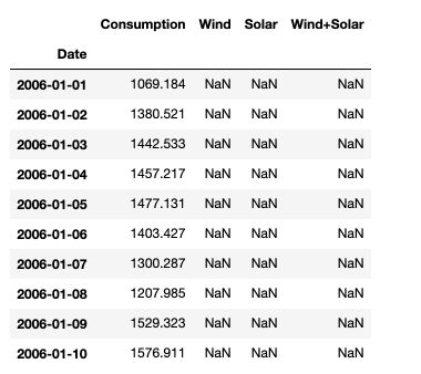
df = pd.read_csv('opsd_germany_daily.csv', index_col=0)
df.head(10)
Then, make sure to transform the dates into datetime format in pandas :
df.index = pd.to_datetime(df.index)
I. Key concepts and definitions
1. Auto-correlation
The auto-correlation \(\rho\) is defined as the correlation of the series over time, i.e how much the value at time \(t\) depends on the value at time \(t-j\) for all \(j\).
- The auto-correlation \(\rho\) of order 1 is : \(Corr(y_t, y_{t-1})\)
- The auto-correlation \(\rho\) of order j is : \(Corr(y_t, y_{t-j})\)
- The auto-covariance \(\rho\) of order 1 is : \(Cov(y_t, y_{t-1})\)
- The auto-covariance \(\rho\) of order j is : \(Cov(y_t, y_{t-j})\)
Empirically, the auto-correlation can be estimated by the sample auto-correlation :
\[r_j = \frac {Cov^e (y_t, y_{t-j})} {Var^e(y_t)}\]Where : \(Cov^e = \frac {1} {T} \sum_{t-j+1} (y_t - \bar{y_{j+1,T}} ) (y_{t-j} - \bar{y_{1,T-j}})\)
To plot the auto-correlation and the partial auto-correlation, we can use statsmodel package :
fig, axes = plt.subplots(1, 2, figsize=(15,8))

fig = sm.graphics.tsa.plot_acf(df['Consumption'], lags=400, ax=axes[0])
fig = sm.graphics.tsa.plot_pacf(df['Consumption'], lags=400, ax=axes[1])
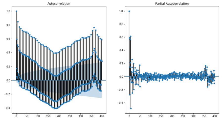
We observe a clear trend. The value od consumption at time \(t\) is negatively correlated with the values 180 days ago, and positively correlated with the values 360 days ago.
2. Partial Auto-correlation
The partial autocorrelation function (PACF) gives the partial correlation of a stationary time series with its own lagged values, regressed the values of the time series at all shorter lags. It is a regression of the series against its past lags.
How can we correct auto-correlation ? Take for example :
\[y_{t-1} = \beta_0 + \beta_1 X_{t-1} + u_{t-1}\] \[y_{t} = \beta_0 + \beta_1 X_{t} + u_{t}\]Therefore, if you substract the first to the second with a coefficient equal to the auto-correlation \(\rho\) :
\(y_t - \rho y_{t-1} = (1-\rho) \beta_0 + \beta_1 (X_t - \rho X_{t-1}) + e_t\) for \(t ≥ 2\)
Therefore, if we want to make a regression without auto-correlation :
\[\hat{y_{t}} = (1-\rho) \beta_0 + \beta_1 \hat{X_t} + e_t\]Why would we want to remove the auto-correlation?
- to derive the OLS estimator of the parameters \(\beta_1\) for example
- because there is a bias otherwise since \(u_t\) would depend on \(u_{t-1}\)
3. Stationarity
Stationarity of a time series is a desired property, reached when the joint distribution of \(y_s, y_{s+1}, y_{s+2}...\) does not depend on \(s\). In other words, the future and the present should be quite similar. Stationary time series do therefore not have underlying trends or seasonal effect.
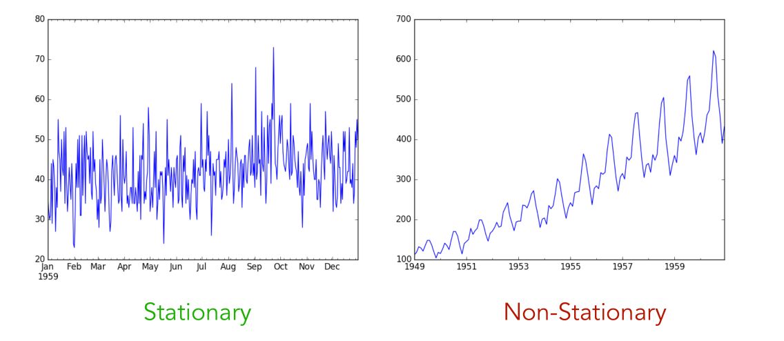
What kind of events makes a series non-stationary?
- a trend, i.e increasing sales over time
- a seasonality, i.e more sales during the summertime than wintertime
We usually want our series to be stationary even before applying any predictive model!
How can we test if a time series is stationary?
- look at the plots (as above)
- look at summary statistics and box plots as in the previous article. A simple trick is to cut the data set in 2, look at mean and variance for each split, and plot the distribution of values for both splits.
- perform statistical tests, using the (Augmented) Dickey-Fuller test
Unit roots
Let’s cover into more details the Dickey-Fuller test. To do so, we need to introduce the notion of unit root. A unit root is a stochastic trend in a time series, sometimes called a random walk with drift. If a series has a unit root, it makes it unpredictable due to a systematic pattern.
Let’s consider an autoregressive (we’ll dive deeper later in to this) :
\[y_t = a_1 y_{t-1} + a_2 y_{t-2} + ... + a_p y_{t-p} + \epsilon_t\]We define the characteristic equation as :
\(m^p - m^{p-1}a_1 - m^{p-2}a_2 - ... - a_p = 0\). If \(m = 1\) is a root to this equation, then the process is said to have a unit root. Equivalently, the process is said to be integrated of order 1 : \(I(1)\).
In other words, there is a unit root if the previous values keep having a 1:1 impact on the current value. If we consider a simple autoregressive model AR(1) : \(y_t = a_1 y_{t-1} + \epsilon_t\), the process has a unit root when \(a_1 = 1\).
If a process has a unit root, then it is non-stationary, i.e the moments of the process depend on \(t\).
A process is a weakly dependent process, also called integrated of order 0 ( \(I(0)\) ) if taking the first different of the model is enough to make the series stationary :
\[\Delta y_t = y_t - y_{t-1}\]Dickey-Fuller Test
The Dicker Fuller test is used to assess if a unit root is present in an autoregressive process :
\(H_0 :\) There is a unit root and the process is not stationary.
\(H_1 :\) There is no unit root and the process is stationary.
For example, in an AR(1) model where \(y_t = \alpha + \rho y_{t-1} + e_t\), the hypothesis are :
\[H_0 : \rho = 1\] \[H_1 : \rho < 1\]The hypothesis \(H_1 > 1\) would mean an explosive process, and is therefore not considered. When \(\mid \rho \mid < 1\), then \(Corr(y_t, y_{t-h}) = \rho^h → 0\).
In practice, we consider the following equation :
\[\Delta y_t = \alpha + \theta y_{t-1} + e_t\]We have \(\theta = \rho -1\) and test \(H_0 : \theta = 0\).
Augmented Dickey-Fuller Test
The Augmented Dickey-Fuller Test (ADF) is an augmented version of the Dickey-Fuller test in the sense that it can test for a more complex set of time series models. For example, consider an ADF on an AR(p) process :
\[\Delta_t = \alpha + \theta y_{t-1} + \gamma_1 \Delta y_{t-1} + ... + \gamma_p \Delta y_{t-p} + \epsilon_t\]And the null hypothesis : \(H_0 : \theta = 0\).
4. Ergodicity
Ergodicity is the process by which we forget the initial conditions. This is reached when auto-correlation of order \(k\) tends to \(0\) as \(k\) tends to \(\infty\).
According to the ergodicity theorem, when a time series is strictly stationary and erdogic, and \(E(Y_T) < \infty\) when \(T → \infty\), then \(\frac {1} {n} \sum_i y_t → E(Y_T)\)
5. Exogeneity
Exogeneity describes the relation between the residuals and the explanatory variables. The exogeneity is said to be strict if :
\(y_t = \beta_0 + \beta_1 X_{t-1} + ... + \beta_k X_{tk} + u_t\) and \(E(u_t \mid X) = 0\) for all t.
The exogenity is said to be contemporary when :
\(E(u_t \mid X_{t-1}, ..., X_{t-k}) = E(u_t \mid X_t) = 0\) which is a weaker assumption, but satisfies the consistency hypothesis.
6. Long term effect
Let’s consider again the model : \(y_t = \beta_0 + \beta_1 X_{t-1} + ... + \beta_k X_{tk} + u_t\). In that case, we can estimate the long term effect as :
\[LRP = \beta_0 + \beta_1 + ... + \beta_q\]We can test the Granger causality using a Fisher test :
\(H_0 : \beta_0 = \beta_1 = ... = \beta_q = 0\). Under this hypothesis, no past value of \(X\) would allow to predict \(Y\).
Conclusion : I hope you found this article useful. Don’t hesitate to drop a comment if you have a question.