
Any parameter estimation requires statistical hypothesis testing. The point of such a test is to assess whether a given parameter is significant or not given the initial hypothesis.
I. Definition and context
Let’s suppose we are interested in the following problem. We want to assess whether the demand for ice cream depends on the outside temperature. The model we would build would look like this :
\[y_i = \beta_0 + \beta_1 * x_i + u_i\]where :
- \(y_i\) is the icecream demand on a given day
- \(\beta_0\) a constant parameter
- \(\beta_1\) the parameter that assesses the impact of temperature on icecream demand
- \(x_i\) the average temparature for a given day
- \(u_i\) the residuals
II. Compute the expectation and the variance
By OLS method, we build an estimator for \(\beta_0\) and \(\beta_1\). We’ll call these estimators \(\hat{\beta}_0\) and \(\hat{\beta}_1\), which can be described by three metrics :
- an expectation
- a bias
- a variance
The expectation of the parameter corresponds… to its expected value. Nothing really new here : \(E(\hat{\beta}_j)\)
The bias corresponds to how far we are from the actual value. It is given by : \(E(\hat{\beta}_j) - {\beta}_j\) . The true bias is typically unknown, as we try to estimate \({\beta}_j\) . If the bias is 0, we say that the estimator is unbiased.
The variance defines the stability of our estimator regarding the observations. Indeed, the features might be highly spread, which would mean a pretty big variance.
It can be shown that the variance of \({\beta}_1\) is given by : \(\hat{\sigma}{_\hat{\beta_1}} = \frac{\hat{\sigma}} {\sqrt{\sum(X_i – \bar{X})^2}}\)
And the one of \({\beta}_0\) by : \(\hat{\sigma}{_\hat{\beta_0}} = \hat{\sigma} \sqrt{\frac{1} {n} + \frac{\sum(X_i)^2} {\sum(X_i – \bar{X})^2}}\)
Where the estimated variance \(\hat{\sigma}\) is defined by : \(\hat{\sigma} = \sqrt\frac{\sum(Y_i – \hat{Y}_i)^2} {n – p-1}\) . This is an unbiaised estimator of the variance.
III. Statistical hypothesis testing
1. Two-sided tests
T-Stat and critical value
For each parameter, we want to test whether the parameter in question has a real impact on the output or not, to avoid adding dimensions that bring no significant information. In the linear regression : \(\hat{Y}_i = \hat{\beta}_0 + \hat{\beta}_1{X}_{i}\) , it would mean testing whether the Betas are significantly different from 0 or not.
To do so, we proceed to a statistical test. If our aim is the state if the parameter is significantly different from 0, we are doing a test with :
- \(H_0\) the null hypothesis : \({\beta}_j = 0\)
- and \(H_1\) the alternative hypothesis : \({\beta}_j ≠ 0\) .
Some further theory is needed here : Recall the Central Limit Theorem. \(\sqrt{n} \frac{\bar{Y}_n - {\mu}} {\sigma}\) converges to \(∼ {N(0,1)}\) as n tends to infinity if \({\sigma}\) is knowm.
In case \({\sigma}\) is unknown, Slutsky’s Lemma states that \(\sqrt{n} \frac{\bar{Y}_n - {\mu}} {\hat{\sigma}}\) converges to \(∼ {N(0,1)}\) if \({\hat{\sigma}}\) converges to \({\sigma}\) .
Most of the time, \({\sigma}\) is unknown. From this point, it can be shown that : \(\hat{T}_j = \frac{\hat{\beta}_j - {\beta}_j} {\hat{\sigma}_j} ∼ {\tau}_{n-p-1}\) where \({\tau}_{n-p-1}\) and \(n-p-1\) is the degrees of freedom (p is the dimension, equal to 1 here).
This metric is called the T-Stat, and it allows us to perform a hypothesis test. The 0 in the numerator can be replaced by any value we would like to test actually.
The T-Stat can be decomposed this way :
- \(\hat{\beta}_j\) is the estimated parameter
- \({\beta}_j\) is the value of the true parameter we are testing
- \(\hat{\beta}_j - {\beta}_j\) follows a Normal distribution
- \({\hat{\sigma}_j}^2 = {\hat{\sigma}^2}_{\hat{\beta_1}}\) follows a Chi Square Distribution
- a ratio of a Normal over the square root of a Chi Square is a Student distribution
How to interpret the T-Stat?
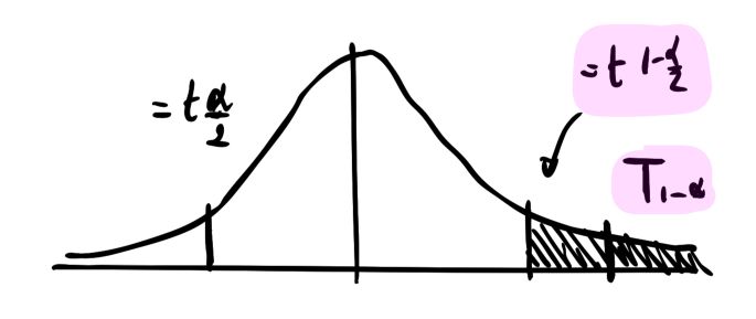
The T-Stat should be compared with the Critical Value. The critical value is the quantile of the corresponding Student distribution at a given level of \({\alpha}\). If a coefficient is significant at a level \({\alpha}\) , this means that the T-Stat is above or under the quantiles of the Student Distribution.
A parameter is said to be significant if its value is significantly different from 0, i.e \(\hat{T}_j = \frac{\hat{\beta}_j - 0} {\hat{\sigma}_j}\) is larger than the critical value.
If the T-Stat is smaller than the critical value, we cannot reject the null hypothesis \(H_0\).
The p-value
Another interpretation is that the probability that the coefficient estimate is not in the interval \([- {t}_{1-{\alpha}/2}; + {t}_{1-{\alpha}/2} ]\) is smaller than \({\alpha}\) . This probability is called the p-value and is defined by :
\[p_{value} = Pr( |\hat{T}_j| > |{t}_{1-{\alpha}/2}|)\]Confidence interval
Using the CLT, one can set a confidence interval around an estimate of a parameter.
The lower bound and the upper bound are determined by the critical value of the student distribution at a level \({\alpha}\), and by the standard deviation of the parameter. \({\beta}_1 ± {t}_{1-{\alpha}/2} * \hat{\sigma}_{\hat{\beta_1}}\)
2. One-sided tests
Implicitely, when we defined the hypothesis to test :
- Null Hypothesis \(H_0\) the null hypothesis : \({\beta}_j = 0\)
- and \(H_1\) the alternative hypothesis : \({\beta}_j ≠ 0\)
we implied a bi-lateral test. Indeed, when we define \(H_1\), we state that both a negative or a positive value of the parameter are considered as failures of \(H_0\).
Now, let’s redefine the hypothesis :
- Null Hypothesis \(H_0 : {\beta}_j = 0\)
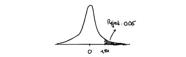
- and \(H_1 : {\beta}_j > 0\)
In this case, we are only interested in one side of the distribution :
III. Joint hypothesis
Let’s add some new variables to our model to explain and predict the icecreams consumption.
\[y_i = \beta_0 + \beta_1 * {X_1}_i + \beta_2 * {X_2}_i + u_i\]1. One parameter against another
Now, what happens if we want to test one parameter against another?
For example, we could define the new hypothesis this way :
- Null Hypothesis \(H_0 : \beta_1 = \beta_2\)
- and \(H_1 : \beta_1 > \beta_2\)
The T-Stat would become :
\[\hat{T}_j = \frac{\hat{\beta}_1 - \hat{\beta}_2} {\hat{\sigma}_{\hat{\beta}_1 - \hat{\beta}_2}}\]The standard deviation is however quite difficult to estimate. For this reason, we define a new parameter : \(\theta_1 = \beta_1 - \beta_2\) . This way, we can just redefine our hypothesis :
- Null Hypothesis \(H_0 : \theta_1 = 0\)
- and \(H_1 : \theta_1 < 0\)
We can replace \(\theta_1\) in our model :
\[y_i = \beta_0 + \beta_1 * {X_1}_i + \beta_2 * {X_2}_i + u_i\] \[y_i = \beta_0 + (\theta_1 + \beta_2) * {X_1}_i + \beta_2 * {X_2}_i + u_i\] \[y_i = \beta_0 + \theta_1 * {X_1}_i + \beta_2 * ({X_2}_i + {X_1}_i) + u_i\]2. Multiple restrictions
We might also want to test several hypothesis at once. For example, in a more complex model :
\[y_i = \beta_0 + \beta_1 * {X_1}_i + \beta_2 * {X_2}_i + \beta_3 * {X_3}_i + \beta_4 * {X_4}_i + u_i\]We might want to test the following joint hypothesis :
- Null Hypothesis \(H_0 : \beta_2 = 0, \beta_3 = 0, \beta_4 = 0\)
- and \(H_1 : H_0\) is not true
The one thing is to avoid using individual student tests. The intuition we rather use is the following: if all the coefficients are not jointly significant, the sum of the squared errors should not diminish if we delete some variables. In other words, under a constrained model where \(\beta_2 = 0, \beta_3 = 0, \beta_4 = 0\), the Sum of Squared Residuals does not change.
Recall that we define the Sum of Squared Residuals (SSR) as :
\[SSR = \sum \hat{u_i}^2\]The constrained model would become :
\[y_i = \beta_0 + \beta_1 * {X_1}_i + u_i\]To test the hypothesis defined above, we define the F-Stat :
\[\hat{F}_j = \frac { \frac { SSR_c - SSR_{uc} } {q} } {\frac {SSR_{uc}} {n-k-1}}\]Where :
- \(SSR_c\) is the sum of squared residuals for the constrained model
- \(SSR_{uc}\) is the sum of squared residuals for the unconstrained model
- \(q\) is the number of restrictions we apply
Under those hypothesis, the F-Stat follows a Fisher distribution : \(\hat{F}_j ∼ {F}_{n-q-1}\)
We can use the Fisher distribution to find the critical value \(C\). As before, we reject \(H_0\) if \(\hat{F}_j > C\).
If we apply only one constraint, the F-Stat is similar to the T-Stat.
**Conclusion **: We have covered the most common tests to apply in the linear regression framework. Don’t hesitate to drop a comment if you have a question.