
David Silver’s YouTube series on Reinforcement Learning, Episode 3.
The full lesson is the following:
We have so far formulated the Bellman Equation, but we did not cover ways to solve it. In this article, we will explore Dynamic Programming, and more specifically:
- policy evaluation
- policy iteration
- value iteration
Dynamic Programming
Dynamic Programming is a very general solution method for problems which have two properties :
- Optimal substructure :
- principle of optimality applies
- optimal solution can be decomposed into subproblems
- Overlapping subproblems :
- subproblems recur many times
- solutions can be cached and reused
Markov Decision Processes satisfy both of these properties. The Bellman equation gives a recursive decomposition. The values function stores and reuses solutions.
Dynamic Programming assumes full knowledge of the MDP. We know the dynamics and the reward. It is used for planning in an MDP, and it’s not a full Reinforcement Learning problem.
For Prediction :
- The input takes the form of an MDP \((S, A, P, R, \gamma)\) and a policy \(\pi\), or an MRP \((S, P^{\pi}, R^{\pi}, \gamma)\).
- The output is a value function \(v_{pi}\).
For Control :
- The input takes the form of an MDP \((S, A, P, R, \gamma)\) and a policy \(\pi\).
- The output is the optimal value function \(v_{*}\), and an optimal policy \(\pi_{*}\).
Dynamic Programming is used in :
- Scheduling algorithms (sequence alignment)
- Graph algorithms (shortest path)
- Graphical models (Viterbi)
- Bioinformatics (lattice models)
- …
Policy Evaluation
If we are given an MDP and a policy (e.g always go straight ahead), how can we evaluate this policy \(\pi\) ?
We apply the Bellman expectation backup iteratively.
We start off with an arbitrary value function \(v_1\). We then do a 1-step look-ahead to figure out \(v_2\). Then, we iterate many times until \(v_{\pi}\).
\[v_1 → v_2 →\cdots → v_{\pi}\]We use synchronous backups :
- At each iteration \(k + 1\) :
- For all states \(s \in S\)
- Update \(v_{k+1}(s)\) from \(v_k(s')\)
- where \(s'\) is a successor state of \(s\)
The convergence of this process can also be proven.
We can represent Policy Evaluation graphically as in the previous article :
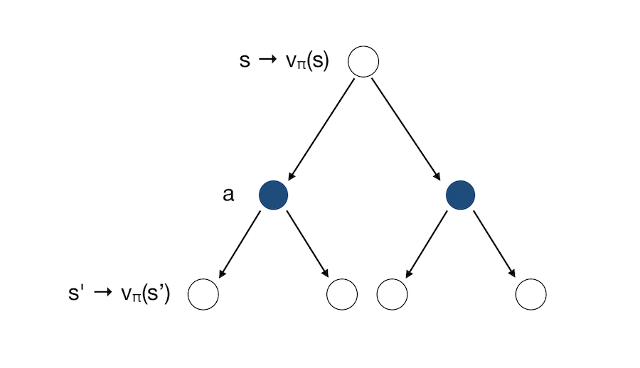
Which can be re-written under matrix form :
\[v^{k+1} = R^{\pi} + \gamma P^{\pi} v^k\]Let us now illustrate this concept with a simple grid. The aim of the agent is to reach one of the terminal states (either upper left or lower right). The reward is \(-1\) until the terminal state is reached.
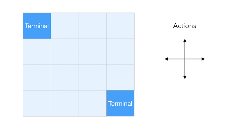
We suppose that the agent follows a uniform random policy, and has \(\frac{1}{4}\) chance to pick each action (Up, Down, Left, Right) :
\[\pi(n \mid .) = \pi(e \mid .) = \pi(s \mid .) = \pi(w \mid .) = 0.25\]Here is what a the greedy policy would look like at step \(0\) of this random policy :
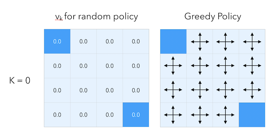
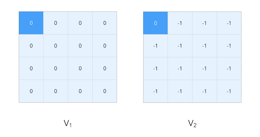
The initial estimate of the value function is to put zeros everywhere. Then, let’s move on by 1 step. For each cell (except for the terminal states), we set the value as a weighted average of the reward we get by following each action. Since the reward is \(-1\) at each cell expect for the terminal states, the average is equal to -1 everywhere.
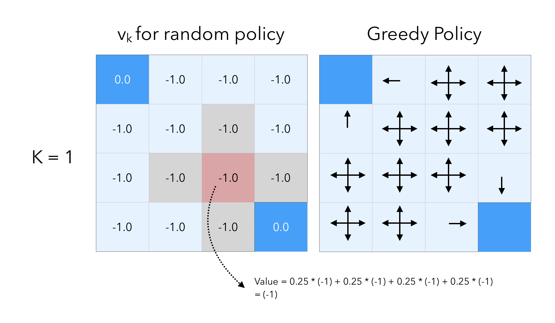
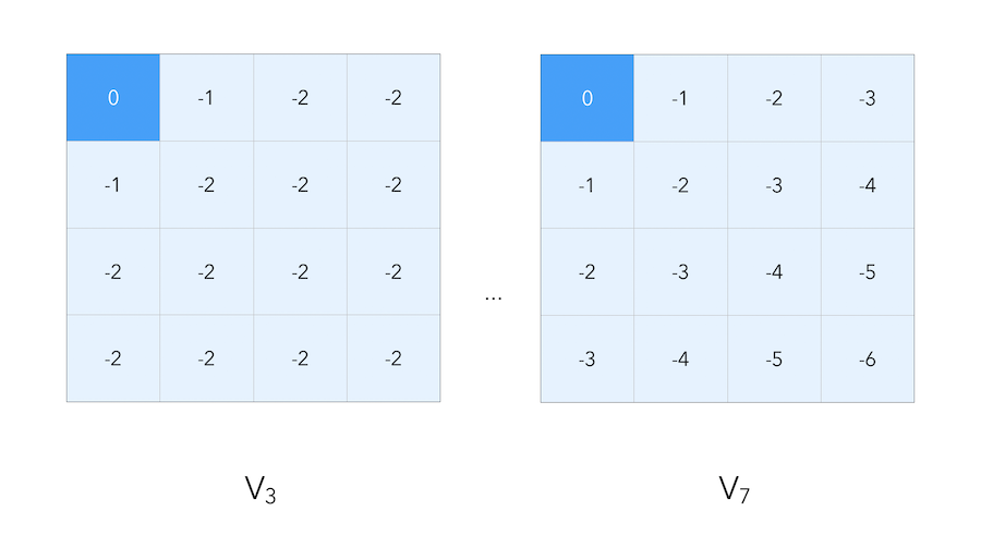
Let’s now move on by 1 step :
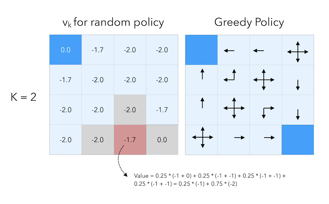
We still get the immediate reward of \(-1\) for moving, but we add to this amount the value of the cell at the previous step. Threfore, by following this principle by which we add the celle value to the reward we get, when we moved from step 0 to step 1, the value of the cells right next to a terminal state is given by:
\[0.25 * (-1 + 0) + 0.25 * (-1 + 0) + 0.25 * (-1 + 0) +0.25 * (-1 + 0) = -1\]If we move by a final step, to \(K = 3\) :
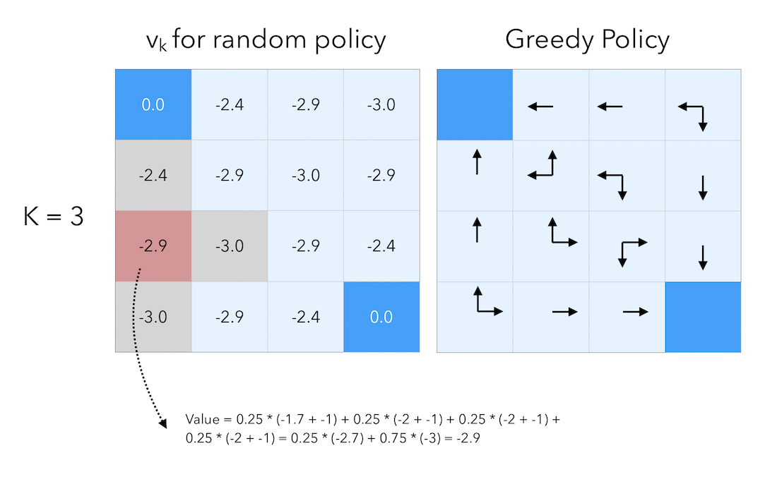
At that point, we have reached the optimal policy. There is no longer need to iterate.
We now have a way to find the value of a given policy iteratively. How do we then identify the optimal policy ?
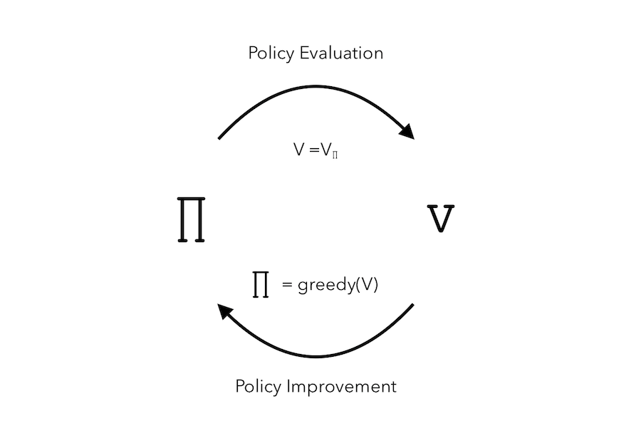
Policy Iteration
Given a policy \(\pi\), how can we improve the policy we used to have ?
- First, evaluate this policy : \(v_{\pi}(s) = E(R_{t+1} + \gamma R_{t+2} + \cdots \mid S_t = s)\)
- Then, improve the policy greedily : \(\pi^{'} = greedy(v_{\pi})\)
The greedy part means that we systematically optimize over the next action by taking into account what will happen if we take this action.
In general, we need a lot of improvements and evaluations. This process of policy iteration always converges to \(\pi^{*}\).
The process can be represented as such :
Let us consider a deterministic policy : \(a = \pi(s)\). We can improve the policy by acting greedily :
\[{\pi}^{'}(s) = argmax_{a \in A}q_{\pi}(s, a)\]This improves the value from any state \(s\) over one step (at lease) :
\[q_{\pi}(s, \pi^{'}(s)) = max_{a \in A}q_{\pi}(s, a) ≥ q_{\pi}(s, \pi(s)) = v_{\p}(s)i\]Therefore, the value function is improved over time :
\(v_{\pi}(s) ≤ q_{\pi}(s, \pi^{'}(s)) = E_{\pi^{'}}(R_{t+1} + \gamma v_{\pi}(S_{t+1}) \mid S_t = s)\) \(≤ E_{\pi^{'}}(R_{t+1} + \gamma q_{\pi}(S_{t+1}, \pi^{'}(S_{t+1})) \mid S_t = s)\) \(≤ E_{\pi^{'}}(R_{t+1} + \gamma R_{t+2} + \gamma^2 q_{\pi}(S_{t+2}, \pi^{'}(S_{t+2})) \mid S_t = s)\) \(≤ E_{\pi^{'}}(R_{t+1} + \gamma R_{t+2} + \cdots \mid S_t = s) = v_{\pi^{'}}(s)\)
What if the improvements stop, i.e :
\[q_{\pi}(s, \pi^{'}(s)) = max_{a \in A} q_{\pi}(s,a) = q_{\pi}(s, \pi(s)) = v_{\pi}(s)\]Have we reached the optimal state? Or a we stuck? We actually satisfy the Bellman optimality equation :
\[v_{\pi}(s) = max_{a \in A} q_{\pi}(s,a)\]Therefore, \(v_{\pi}(s) = v_{*}(s)\) for all \(s \in S\).
And \(\pi\) is the optimal policy.
Policy iteration solves MDPs. If the iteration ever stops, it means that the optimal policy has been identified.
Modified Policy Iteration
Sometimes, we do not need the policy iteration to converge to \(v_{\pi}\) exactly, since this process might be really long. We can therefore :
- introduce a stopping criteria over an \(\epsilon\) convergence
- stop after \(k\) iterations
This is called the modified policy iteration.
Value Iteration
Principle of optimality : A policy \(\pi(a \mid s)\) achieves the optimal value from state \(s\), \(v_{\pi}(s) = v_{*}(s)\) if and only if for any state \(s^{'}\) reachable from \(s\), \(\pi\) achieves the optimal value state \(s^{'}\) : \(v_{\pi}(s') = v_{*}(s')\)
Suppose that we know the solution to subproblems \(v_{*}(s')\). Using Bellman, the solution \(v_{*}(s)\) can be found by one-step lookahead :
\[v_{*}(s) = max_{a \in A} R_s^a + \gamma \sum_{s' \in S} P_{ss'}^a v_{*}(s')\]The idea of value iteration is to apply these updates iteratively.
We start with the final rewardds, and work backwards. Suppose that we work on a small gridworld again, where our goal is to reach the blue top-left corner.
As before, we suppose that moving has a reward of \(-1\), and reaching the final state has a reward of \(0\). When we compute the value iteration, we propagate the reward step by step :
In value iteration, we must find optimal policy \(\pi\) by iteratively applying Bellman optimality backup : \(v_1 → v_2 →\cdots → v_{*}\)
It relies on synchronous backups :
- At each state \(k+1\)
- For all states \(s \in S\)
- Update \(v_{k+1}(s)\) from \(v_k(s')\)
Unlike policy iteration, there is no explicit policy.