Markov Decision Process

David Silver’s YouTube series on Reinforcement Learning, Episode 2.

The full lesson is the following:

A Markov Decision Process descrbes an environment for reinforcement learning. The environment is fully observable. In MDPs, the current state completely characterises the process.

Markov Process (MP)

The Markov Property states the following:

A state \(S_t\) is Markov if and only if \(P(S_{t+1} \mid S_t) = P(S_{t+1} \mid S_1, ..., S_t)\)

The transition between a state \(s\) and the next state \(s'\) is characterized by a transition probability. It is defined by :

\[P_{ss'} = P(S_{t+1} = s' \mid S_t = s)\]

We can characterize a state transition matrix \(P\), describing all transition probabilities from all states \(s\) to all successor states \(s'\), where each row of the matrix sums to 1.

\[P = \begin{bmatrix} P_{11} & \cdots & P_{1n} \\ \cdots & \cdots & \cdots \\ P_{n1} & \cdots & P_{nn} \\ \end{bmatrix}\]

A Markov Process is a memoryless random process. It is a sequence of randdom states \(S_1, S_2, \cdots\) with the Markov Property.

A Markov Process, also known as Markov Chain, is a tuple \((S,P)\), where :

• \(S\) is a finite set of states
• \(P\) is a state transition probability matrix such that \(P_{ss'} = P(S_{t+1} = s' \mid S_t = s)\)

We can represent a Markov Decision Process schematically the following way :

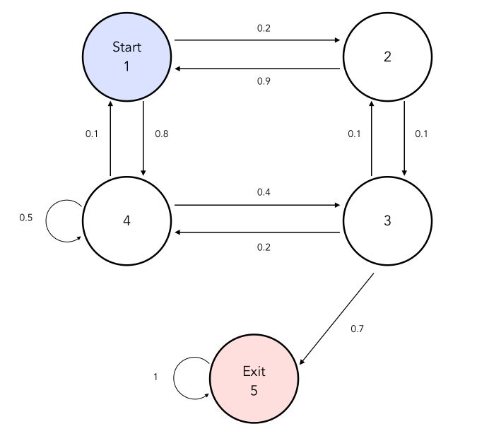
Samples describe chains that take different states. For example, it could be :

• 1, 1, 2, 1, 2, 3, 4, 3, Exit
• 1, 2, 3, Exit
• …

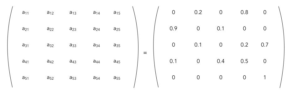
The transition matrix corresponding to this problem is :

Markov Reward Process (MRP)

Markov Reward

A Markov Reward is a Markov Chain a value function. A Markov Reward Process is a tuple \((S, P, R, \gamma)\) where :

• \(R\) is a reward function \(R_s = E(R_{t+1} \mid S_t = s)\)
• \(\gamma\) is a discount factor between 0 and 1
• all other components are the same as before

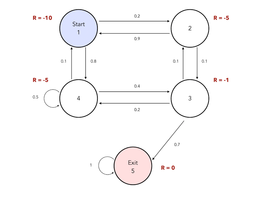
We can therefore attach a reward to each state in the following graph :

Then, the Return is the total discounte reward from time-step \(t\) :

\[G_t = R_{t+1} + \gamma R_{t+2} + \cdots = \sum_{k=0} \gamma^k R_{t+k+1}\]

Just like in Finance, we compute the present value of future rewards. This represents the fact that we prefer to get reward now instead of getting it in the future.

• if \(\gamma\) is close to 0, we have a “myopic” evaluation where almost only the present matters
• if \(\gamma\) is close to 1, we have a “far-sighted” evaluation

A simple return for the sequence 1-1-2-3-Exit and with \(\gamma = 0.8\) would be :

\[G_1 = (-10) + (-10) * 0.8 + (-5) * 0.8^2 + (-1) * 0.8^3\]

But why do we use a discount factor ?

• there is uncertainty in the future, and our model is not perfect
• it avoids infinite returns in cyclical Markov Processes
• animals and humans have a preference for immediate reward

Bellman Equation

The value function \(v(s)\) gives the long-term value of a state \(s\). It reflects the expected return when we are in a given state :

\[v(s) = E(G_t \mid S_t = s)\]

The value function can be decomposed in two parts :

• the immediate reward \(R_{t+1}\)
• the discounted value of the successor rate \(\gamma v(S_{t+1})\)

This is the Bellman Equation for MRP :

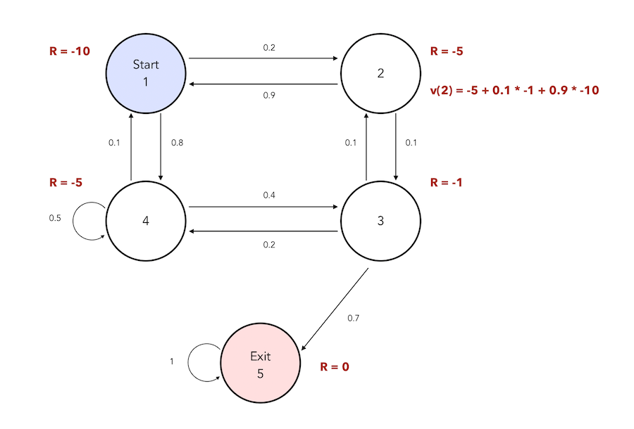
\[v(s) = E(G_t \mid S_t = s) = E(R_{t+1} + \gamma R_{t+2} + \cdots \mid S_t = s)\] \[= E(R_{t+1} + \gamma(R_{t+2} + \gamma R_{t+3} + \cdots) \mid S_t = s\] \[= E(R_{t+1} + \gamma G_{t+1} \mid S_t = s) = E(R_{t+1} + \gamma v(S_{t+1}) \mid S_t = s)\] \[= R_s + \gamma \sum_{s' \in S} P_{ss'} v(s')\]

If we consider that \(\gamma\) is equal to 1, we can compute the value function at state 2 in our previous example :

We can summarize the Bellman equation is a matrix form :

\[v = R + \gamma P v\] \[\begin{bmatrix} v(1) \\ \cdots \\ v(n) \\ \end{bmatrix} = \begin{bmatrix} R_1 \\ \cdots \\ R_n \\ \end{bmatrix} + \gamma \begin{bmatrix} P_{11} & \cdots & P_{1n} \\ \cdots & \cdots & \cdots \\ P_{n1} & \cdots & P_{nn} \\ \end{bmatrix} \begin{bmatrix} v(1) \\ \cdots \\ v(n) \\ \end{bmatrix}\]

We can solve this equation as a simple linear equation :

\[v = R + \gamma P v\] \[(1 - \gamma P) v = R\] \[v = (1 - \gamma P)^{-1} R\]

However, solving this equation this way has a computational complexity of \(O(n^3)\) for \(n\) states since it contains a matrix inversion step. There are several ways to compute it faster, and we’ll develop those solutions later on.

Markov Decision Process (MDP)

So far, we have not seen the action component. Markov Decision Process (MDP) is a Markov Reward Process with decisions. As defined at the beginning of the article, it is an environment in which all states are Markov.

A Markov Decision Process is a tuple of the form : \((S, A, P, R, \gamma)\) where :

• \(A\) is a finite set of actions
• \(P\) the state probability matrix is now modified : \(P_{ss'}^a = P(S_{t+1} = s' \mid S_t = s, A_t = a)\)
• \(R\) the reward function is now modified : \(R_s^a = E(R_{t+1} \mid S_t = s, A_t = a)\)
• all other components are the same as before

We now have more control on the actions we can take :

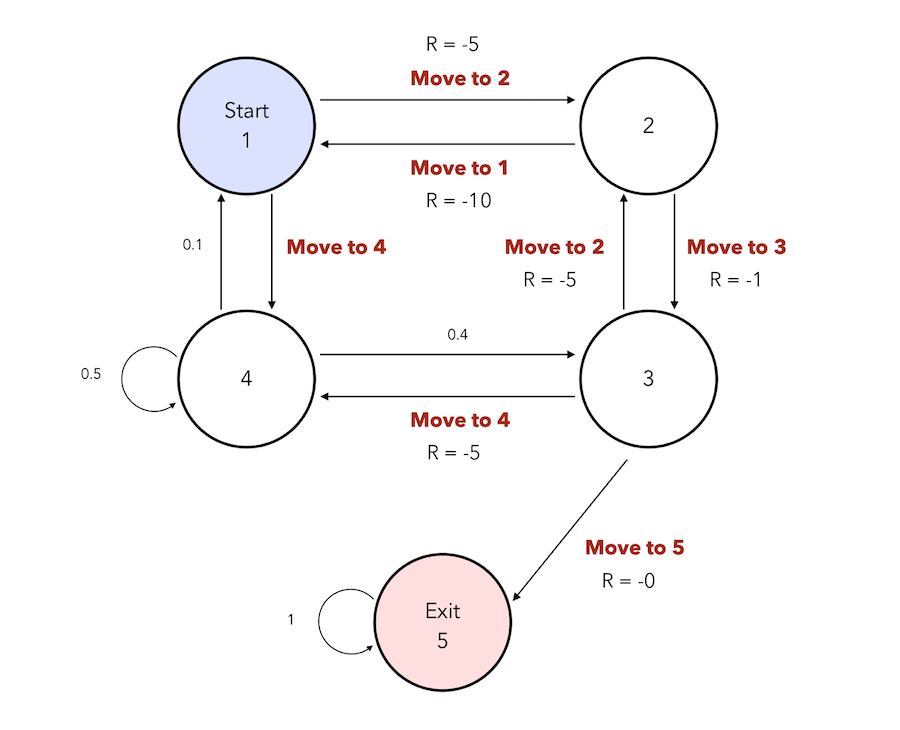
There might stil be some states in which we cannot take action and are subject to the transition probabilities, but in other states, we have an action choice to make. This is the reality of an agent, and we needd to maximize the reward and find the best path to reach the final state.

But what does it mean to actually make a decision ?

Policies

The agent chooses a policy. A policy \(\pi\) is a distribution over actions given states.

\[\pi(a \mid s) = P(A_t = a \mid S_t = s)\]

A policy describes the behavior of an agent. Policies are time stationary, they donnot depend on time.

\[A_t \sim \pi(. \mid S_t)\]

Given an MDP \(M = (S, A, P, R, \gamma)\) and a policy \(\pi\) :

• the state sequence \(S_1, S_2, \cdots\) is a Markov Process \((S, P^{\pi})\).
• the state and reward sequence \(S_1, R_2, S_2, \cdots\) is a Markov Reward Process \((S, P^{\pi}, R^{\pi}, \gamma)\).

We compte the Markov Reward Process values by averaging over the dynamics that result of each choice. In other words :

\[P_{s,s'}^{\pi} = \sum_{a \in A} \pi(a \mid s) P_{s,s'}^a\] \[R_{s}^{\pi} = \sum_{a \in A} \pi(a \mid s) R_{s}^a\]

Value Function

The state-value function \(v_{\pi}(s)\) of an MDP is now conditional to the chosen policy \(\pi\). It is the expected return starting from state \(s\) and following policy \(\pi\) :

\[v_{\pi}(s) = E_{\pi}(G_t \mid S_t = s)\]

The action-value function \(q_{\pi}(s, a)\) is the expected return starting from a state \(s\), taking action \(a\) and following policy \(\pi\) :

\[q_{\pi}(s,a) = E_{\pi}(G_t \mid S_t = s, A_t = a)\]

The state-value function can again be decomposed into immediate reward plus discounted value of successor rate. This is the Bellman Expectation Equation :

\[v_{\pi}(s) = E_{\pi} (R_{t+1} + \gamma v_{\pi}(S_{t+1}) \mid S_t = s)\]

The action-value function can be decomposed similarly :

\[q_{\pi}(s, a) = E_{\pi} (R_{t+1} + \gamma q_{\pi}(S_{t+1}, A_{t+1}) \mid S_t = s, A_t = a)\]

Let’s illustrate those concepts ! Suppose we start in the state \(s\). We can take actions, either the one on the left or on the right. To each action, we attach a q-value, which gives the value of taking this action. The value of being in state \(s\) is therefore an average of both actions :

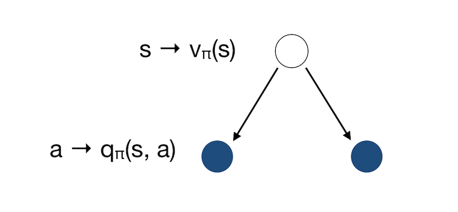
This is the Bellman Expectation Equation for \(v_{\pi}\) :

\[v_{\pi}(s) = \sum_{a \in A} \pi (a \mid s) q_{\pi}(s,a)\]

What if we now consider the inverse ? We start from an action, and have two resulting states.

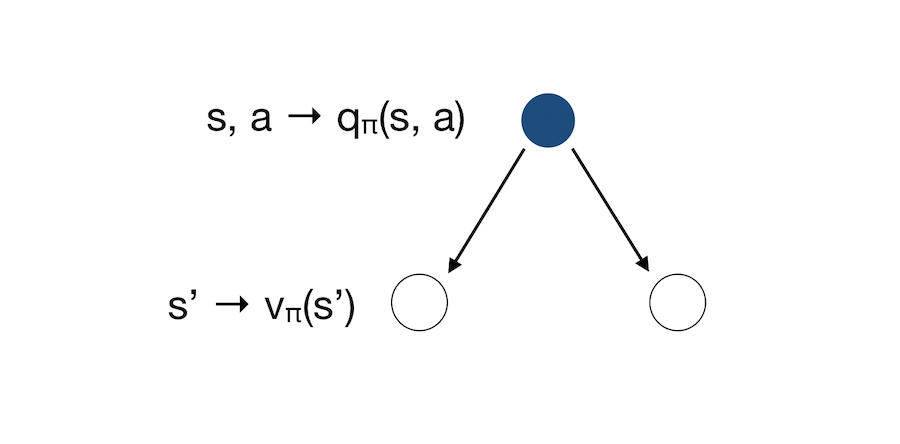
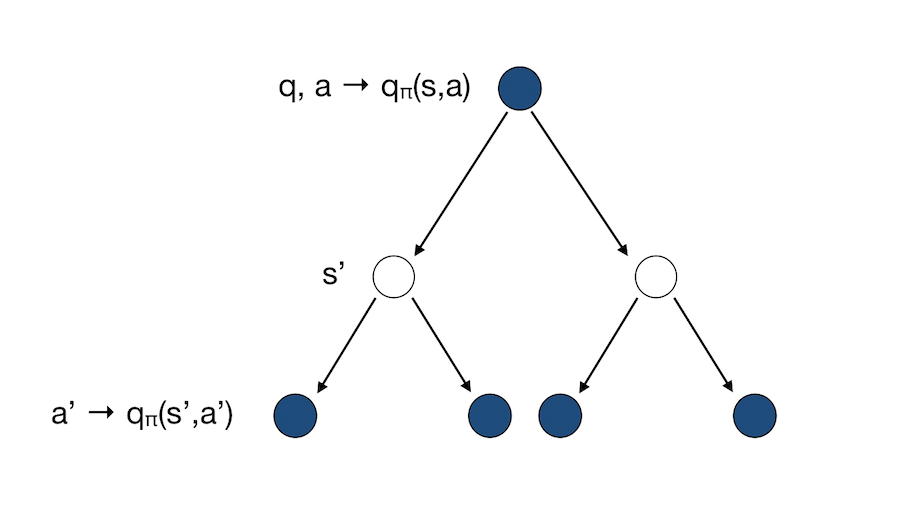
The state shows how good it is to be in a state. The action tells us how good it is to take an action. This is the Bellman Expectation Equation for \(q_{\pi}\) :

\[q_{\pi}(s, a) = R_s^a + \gamma \sum_{s \in S} P_{ss'}^a v_{\pi}(s')\]

We can now group both interpretations into a single graph :

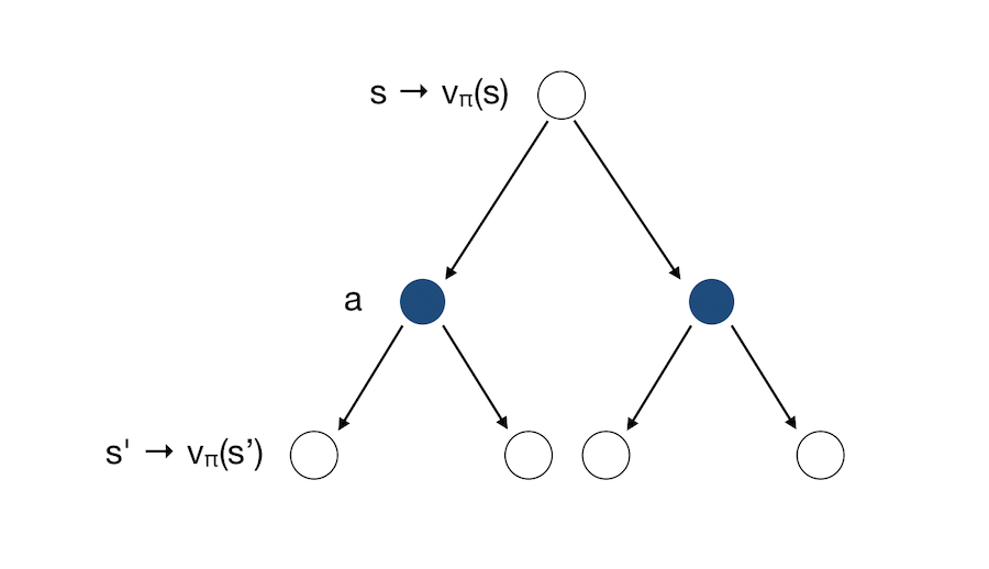
This shows us a recursion that expresses \(v\) in terms of itself. This is how we solve the Markov Decision Process. At the root of the tree, we know how gooddit is to be in a state. We then consider all the actions we might do given the policy. For each action, there are possible outcome states.

We can now express the Bellman Equation a for the state-value as :

\[v_{\pi}(s) = \sum_{a \in A} \pi (a \mid s) (R_s^a + \gamma \sum_{s' \in S} P_{ss'}^a v_{\pi}(s'))\]

And similarly for the action-value :

\[q_{\pi}(s, a) = R_s^a + \gamma \sum_{s' \in S} P_{ss'}^a \sum_{a' \in A} \pi(a'\mid s') q_{\pi}(s', a')\]

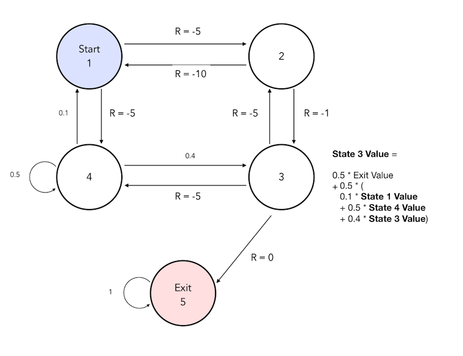
We can simply illustrate how this Bellman Expectation works. We suppose here that there is no discount, and that our policy is to pick each action with a probability of 50%.

We can represent the Bellman Expectation Equation in a matrix form :

\[v_{\pi} = R^{\pi} + \gamma P^{\pi}v_{\pi}\]

The solution is given by :

\[v_{\pi} = (1 - \gamma P^{\pi})^{-1} R^{\pi}\]

Again, the inversion of the matrix is of complexity \(O(n^3)\), and we there need more efficient ways to solve this.

Optimal Value Function

The optimal state-value function \(v_{*}(s)\) is the maximum value function over all policies : \(v_{*}(s) = max_{\pi} v_{\pi}(s)\)

It reflects the maximum reward we can get by following the best policy.

The optimal action-value function \(q_{*}(s, a)\) is the maximum action-value function over all policies. \(q_{*}(s, a) = max_{\pi} q_{\pi}(s, a)\)

It shows given that we commit to a particular action in state \(s\), what is the maximum reward we can get.

An optimal value function specifies the best possible performance in the MDP. An MDP is said to be solved if we know the optimal value function.

Optimal Policy

The optimal policy defines the best possible way to behave in an MDP. We first define a partial ordering over policies :

\(\pi ≥ \pi^'\) if \(v_{\pi}(s) ≥ v_{\pi^'}(s)\)

For any MDP, there exists an optimal policy \(\pi\) that is better than or equal to all other policies.

• All optimal policies achieve the optimal value function : \(v_{\pi^*}(s) = v_{*}(s)\)
• All optimal policies achieve the optimal action-value function : \(q_{\pi^*}(s, a) = q_{*}(s, a)\)

So, how do we find this policy ? We must maximise over \(q_{*}(s, a)\) :

\(\pi_{*}(a \mid s) = 1\) if \(a = argmax_{a \in A} q_{*}(s, a)\), and \(0\) otherwise.

This tells us that once we have found \(q_{*}(s, a)\), we are done. This now brings the problem to : How do we find \(q_{*}(s, a)\) ?

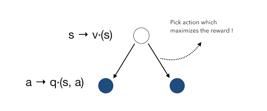
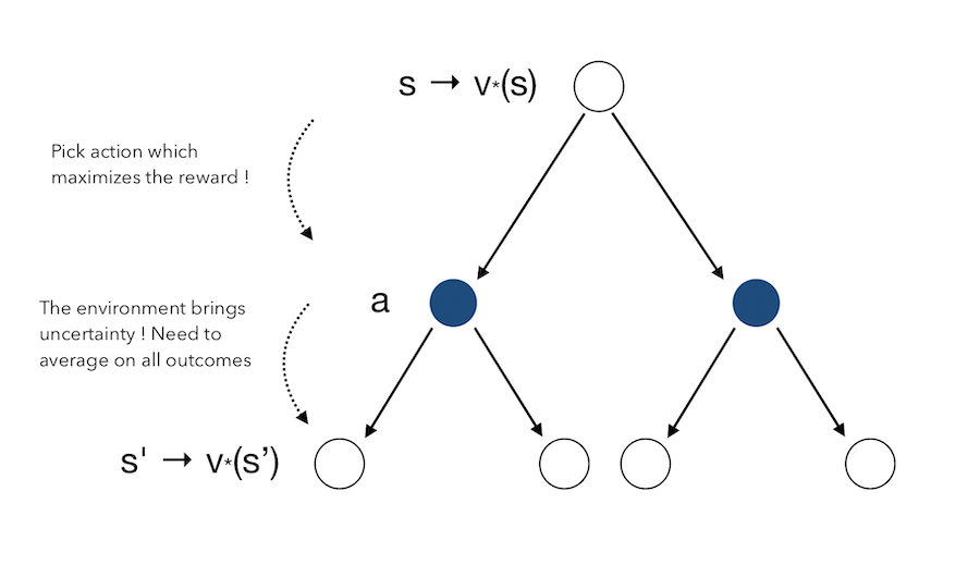
Once we are in the final state, it’s quite easy. We know which action will lead to the maximal reward. If we move back to one state before, we know that the state we were in leads to the maximum reward. We therefore pick this action since it maximizes the reward. If we move another step before, we …

You get the idea. This simply means that we can move backward, and take at each state the action that maximizes the reward :

\[v_{*}(s) = max_a q_{*}(s,a)\]

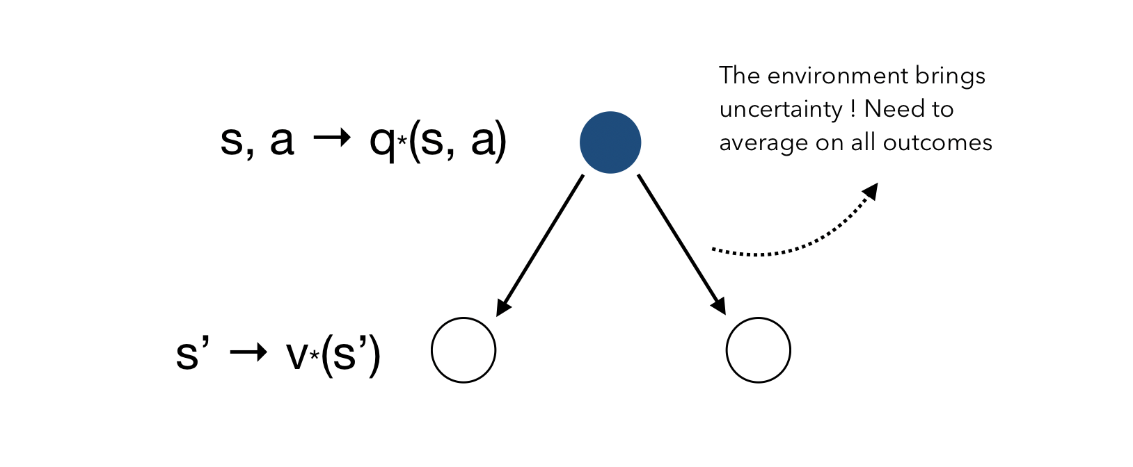
However, when picking an action, we must average over what the environment might do to us once we have picke this action.

\[q_{*}(s,a) = R_s^a + \gamma \sum_{s \in S} P_{ss'}^a v_{*}(s')\]

The Bellman Optimality Equation for \(V^*\) can be obtained by combining both :

\[v_{*}(s) = max_a R_s^a + \gamma \sum_{s' \in S} P_{ss'}^a v_{*}(s')\]

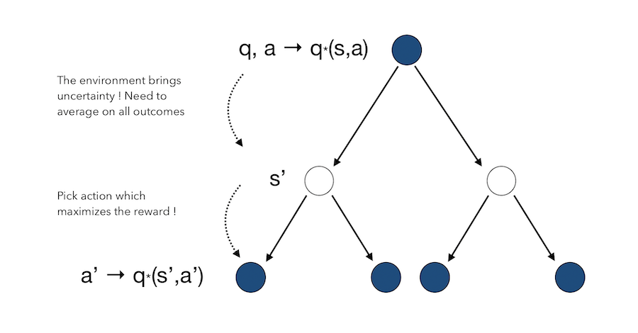
And finally, we can switch the order andd start with the action to derive the Bellman Equation for \(Q^*\). We start by taking the action \(a\), and there is an uncertainty on the state the environment is going to lead us in. Then, wherever we are, we get to make a decision to maximise the reward.

\[q_{*}(s,a) = R_s^a + \gamma \sum_{s' \in S} P_{ss'}^a max_{a'} q_{*}(s', a')\]

Solving the Bellman Equation

The Bellman Equation is a non-linear problem. There is no closed form solution in general. We need to use iterative solutions, among which :

• value iteration
• policy iteration
• Q-learning
• Sarsa

Value and policy iteration are Dynamic Programming algorithms, and we’ll cover them in the next article.