
I was recently recommended to take a look at David Silver’s (from DeepMind) YouTube series on Reinforcement Learning. The whole course (10 videos) can be found here.
The full lesson is the following:
In this series, I am going to :
- summarize the important notions taught in each class
- add examples and code
- illustrate some concepts with home made schemas
- do a Deep RL project
- go a bit further by exploring Twin Delayed DDPG and other SOTA models
Introduction to RL
Reinforcement Learning is at the intersection of many fields of science :
- Machine Learning
- Reward System
- Classical/Operant conditioning
- Bounded Rationality
- Operations Research
- Optimal Control
How is RL different from other ML paraddigms ?
- There is no supervisor, only a reward signal
- Feedback is delayed, not instantaneous
- Time matters, since we consider sequences
- The agent’s actions affect the data it sees
Where is RL applied ?
- manage an investment portfolio
- make a robot walk
- control a power station
- play games (Atari, Go…)
Here is a simulation environment in which we trained an agent to run :
The RL learning problem
A reward \(R_t\) is a feedback value. In indicates how well the agent is doing at step \(t\). The job of the agent is to maximize the cumulative reward.
Reward Hypothesis : All goals can be described by the maximisation of expected cumulative reward.
Some reward examples :
- give reward to the agent if it defeats the Go champion
- give reward to the agent for each dollar that gets in the bank (investment portfolio)
- give reward to the agent if the score of the game increases
- …
The reward might be at the end of the whole process, or at each step, depending on the type of problem we consider.
The environment
This is a Sequential Decision Making process. We select actions to maximise the total future reward.
Actions can have long term consequences, and the reward might be delayed. It may be better to sacrifice immediate reward to gain more long-term reward.
- The agent makes an observation \(O_t\).
- The agent then takes action \(A_t\).
- Based on this action, it gets a reward \(R_t\).
- There is a new environment, and a new observation is made
It can be represented in the following way :
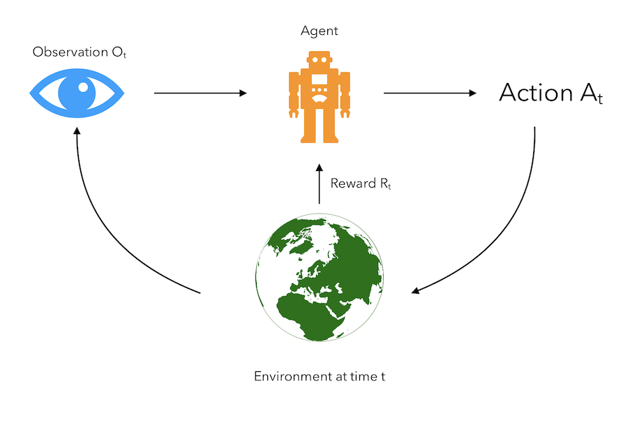
The only leverage the agent has on its environment and the reward it gets is the action it takes.
History and State
The history is the sequence of observations, actions and rewards. It’s all the observable variables up to time \(t\) : \(H_t = A_1, O_1, R_1, \cdots, A_t, O_t, R_t\)
What happens next depends on this history. Our aim is simply to find the right action to take based on the history.
We don’t always use the whole history. Instead, we use the state. It is the information that is used to determine what happens next. It captures all necessary information, and is a function of the history.
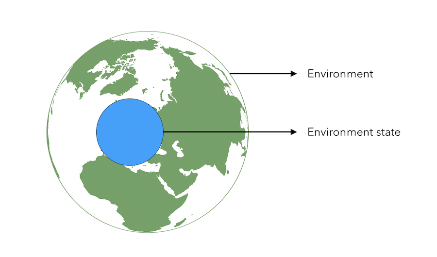
\[S_t = f(H_t)\]The environment state is what is used inside of the environment to determine what should come next : \(S_t^e\).
If you want to go from A to B, to decide where to turn, you don’t need a map of the whole world, but simply things that are relevant around you. This is the idea behind environment state.
The environment state is however not usually visible to the agent. An agent being in an environment state does not mean that the agent gets data from the whole environment around him or captures data from this whole environment. Only the observations are sent to the agent.
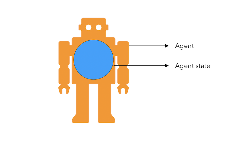
The agent state \(S_t^a\) is the agent’s internal representation. It is all the information used by the agent to take the action. It is a function of the history : \(S_t^a = f(H_t)\)
The environment state and the agent state are both information states. An information state is a Markov State. It contains all information from the history :
A state \(S_t\) is a Markov State if and only if \(P(S_{t+1} \mid S_t) = P(S_{t+1} \mid S_1, ..., S_t)\)
Once a state is known, the history may be thrown away. The current state is a sufficient statistic of the future. The environment state \(S_t^e\) is Markov. The history \(H_t\) is Markov.
A fully observable environment is an environment in which the agent directly observes the environment state : \(O_t = S_t^a = S_t^e\). This is a Markov Decision Process (MDP).
A partially observed environment is an environment in which the agent indirectly observes the environment. This could be the casr for a robot with limited vision, a trading agent that only knows the current prices… This is called a Partially Observed Markov Decision Process (POMDP). The agent must then construct its own state representation \(S_t^a\), either by :
- taking the complete history : \(S_t^a = H_t\)
- beliefs of environment state : \(S_t^a = (P(S_t^e = s^1), \cdots, P(S_t^e = s^e))\)
- recurrent neural network : \(S_t^a = \sigma(S_{t-1}^a W_s + O_t W_o)\)
The RL Agent
An RL agent includes one or more of these components :
- Policy : agent’s bevavior function
- Value function : how good is each state and/or action
- Model : Agent’s representation of the environment
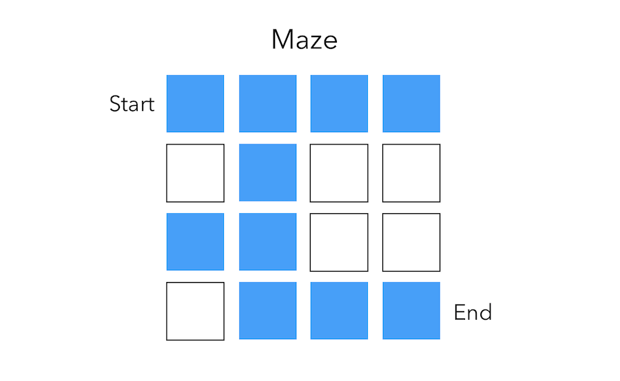
To illustrate those concepts, suppose that we are facing a really simple maze and want to go from the start position to the end by shifting by at most 1 square each time.
Policy
The policy is the agent’s behavior. It maps the state to the action. The policy can be :
- deterministic : \(a = \pi(s)\)
- stochastic : \(\pi(a \mid s) = P(A=a \mid S=s)\)
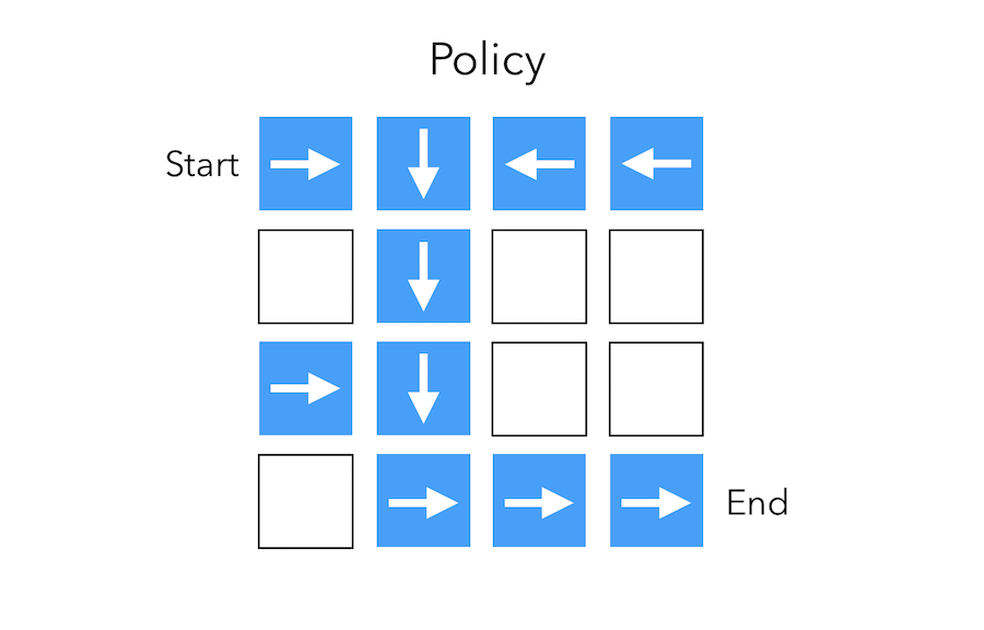
The arrows represent the policy \(\pi(s)\) for each state \(s\).
Value function
The value function is a prediction of expected future reward. It depends on the way we are behaving, and therefore on \(\pi\).
\[V_{\pi}(s) = E_{\pi}(R_t + \gamma R_{t+1} + \gamma^2 R_{t+2} + \cdots \mid S_t = s )\]The value function for a policy gives us the total reward we expect by selecting this policy. It is the sum of the discounted rewards associated to a specific policy.
For example, in the maze example, we could attach the value -1 to the goal, and remove 1 at each step. Some paths as the upper right one are therefore not optimal since the value diminishes.
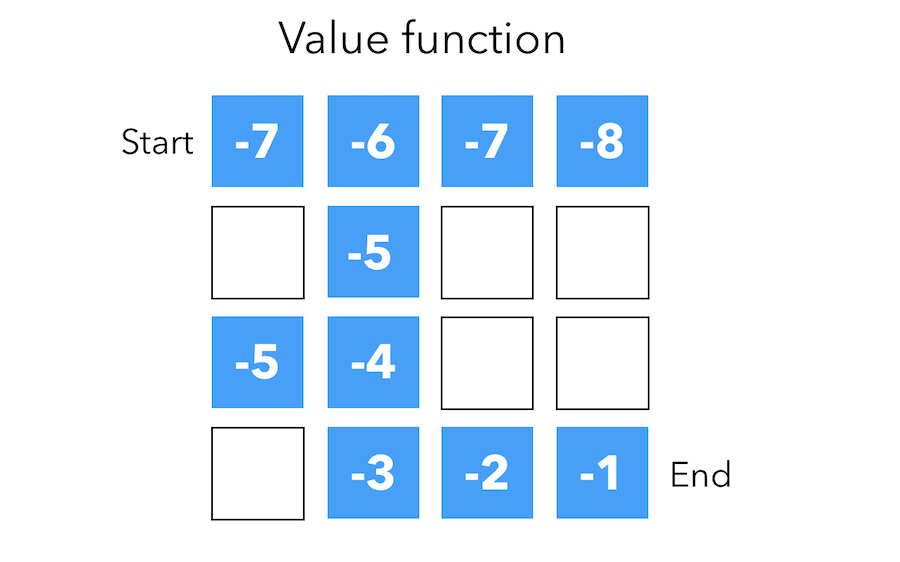
The numbers represent value \(v_{\pi(s)}\) of each state \(s\).
Model
A model predicts what the environment will do next. The transitions \(P\) predicts the next state.
\[P_{ss'}^a = P(S' = s' \mid S = s, A = a)\]The rewards \(R\) predicts the next reward :
\[R_{s}^a = E(R \mid S = s, A = a)\]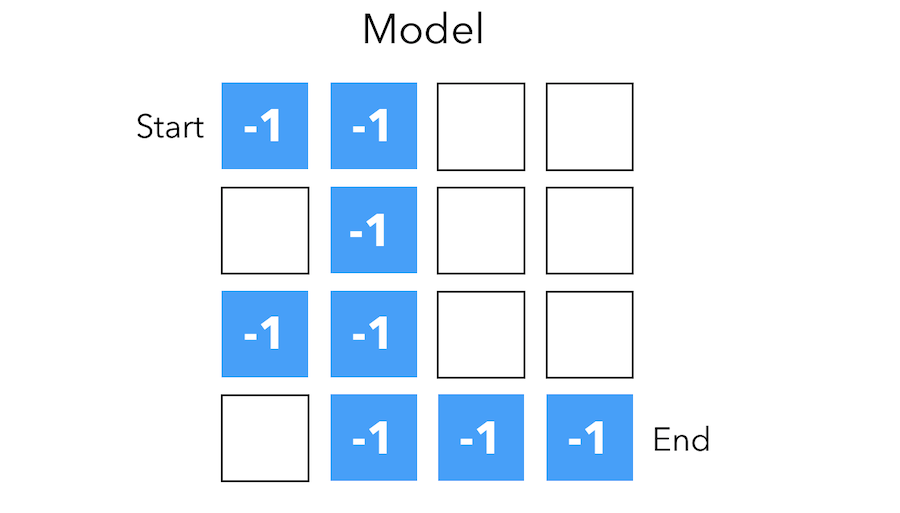
The grid layout represents transition model \(P_{ss'}^a\). The numbers represent immediate reward \(R_s^a\) from each state (same for all action). This is a 1 step prediction of the reward, and describes what the agent understood of the environment.
The reward can however be different for each action.
There is not always a model in the environment. In such case, we talk of model-free environments.
Taxonomy
A RL agent can be :
- Value Based : works with the value function itself. No policy (implicit)
- Policy Based : works with the arrows directly, in a structured way, and tries to adjust it. No value function.
- Actor Critic : combines both value andd policy based.
A RL agent can be :
- Model Free : Policy and/or value function. We do not model the environment around a helicopter for example.
- Model Based : Policy and/or value function, but has a model.
Problems in RL
There are 2 fundamental problems in sequential decision making :
- Reinforcement learning : the environment is initially unknows, the agents interacts with the environment and it improves its policy.
- Planning : a model of the environment is known, the agent performs computations with its model and improves its policy.
Planning can be seen as a tree-based search to find the optimal policy.
Reinforcement Learning is a trial and error learning problem. The agent should discover a good policy wthout losing too much reward.
An RL agent must balance between Exploration and Exploitation.
Exploration finds more information about the environment. Exploitation exploits known information to maximise the reward.