Create an Auto-Encoder

5 minute read

Autoencoder is a type a neural network widely used for unsupervised dimension reduction. So, how does it work? What can it be used for? And how do we implement it in Python?

The origins of autoencoders have been discussed, but one of the most likely origins of the autoencoder is a paper written in 1987 by Ballard, “Modular Learning in Neural Networks” which can be found here.

What is an autoencoder?

An autoencoder is a special type of neural network architecture that can be used efficiently reduce the dimension of the input. It is widely used for images datasets for example.

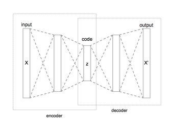
Let’s consider an input image. The input will be sent into several hidden layers of a neural network. Those layers are used to compress the image into a smaller dimension, by reducing the dimensions of the layers as we move on. At some point, the input image will be encoded into a short code.

On the other hand, we build new layers that will learn to decode the short code, to rebuild the initial image. We are now teaching a network to take an input image, reduce its dimension (encoding), and rebuild it on the other side (decoding).

The network will learn by itself to gather the most important information in the short code.

Therefore, all we need to do is to keep the encoding part of the model, and we have a great way to reduce the input dimension in an unsupervised way!

We can summarize the network architecture as follows :

With an image dataset, the layers that are usually used are the following :

convolution layers
activation layers
max-pooling layers
upsampling layers

Otherwise, with numerical problems, dense layers are simple to use.

“If linear activations are used, or only a single sigmoid hidden layer, then the optimal solution to an autoencoder is strongly related to principal component analysis (PCA). The weights of an autoencoder with a single hidden layer of size p (where p is less than the size of the input) span the same vector subspace as the one spanned by the first p principal components, and the output of the autoencoder is an orthogonal projection onto this subspace. The autoencoder weights are not equal to the principal components and are generally not orthogonal, yet the principal components may be recovered from them using the singular value decomposition” (Wikipedia)

Variations

Autoencoder can also be used for :

Denoising autoencoder Take a partially corrupted input image, and teach the network to output the de-noised image.
Sparse autoencoder In a Sparse autoencoder, there are more hidden units than inputs themselves, but only a small number of the hidden units are allowed to be active at the same time. This makes the training easier.
Concrete autoencoder A concrete autoencoder is an autoencoder designed to handle discrete features. In the latent space representation, the features used are only user-specifier.
Contractive autoencoder Contractive autoencoder adds a regularization in the objective function so that the model is robust to slight variations of input values.
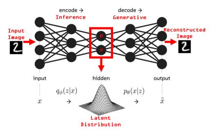
Variational autoencoder (VAE) Variational autoencoders (VAEs) don’t learn to morph the data in and out of a compressed representation of itself. Instead, they learn the parameters of the probability distribution that the data came from. These types of autoencoders have much in common with latent factor analysis.

Create an autoencoder in Python

For this example, we’ll use the MNIST dataset. Start by importing the following packages :

### General Imports ###
import pandas as pd
import numpy as np
import matplotlib.pyplot as plt

### Autoencoder ###
import tensorflow as tf
import tensorflow.keras

from tensorflow.keras import models, layers
from tensorflow.keras.models import Model, model_from_json

from tensorflow.keras.layers import Dense, Dropout, Activation, Flatten, Conv2D, MaxPooling2D, UpSampling2D, Input

from tensorflow.keras.datasets import mnist

Then, load and reshape the data :

(X_train, _), (X_test, _) = mnist.load_data()
shape_x = 28
shape_y = 28

X_train = X_train.astype('float32') / 255.
X_test = X_test.astype('float32') / 255.

X_train = X_train.reshape(-1,shape_x,shape_y,1)
X_test = X_test.reshape(-1,shape_x,shape_y,1)

Now, let’s build the model!

input_img = Input(shape=(shape_x, shape_y, 1))

# Ecoding
x = Conv2D(16, (3, 3), padding='same', activation='relu')(input_img)
x = MaxPooling2D(pool_size=(2,2), padding='same')(x)
x = Conv2D(1,(3, 3), padding='same', activation='relu')(x)
encoded = MaxPooling2D(pool_size=(2,2), padding='same')(x)

# Decoding
x = Conv2D(1,(3, 3), padding='same', activation='relu')(encoded)
x = UpSampling2D((2, 2))(x)
x = Conv2D(16,(3, 3), padding='same', activation='relu')(x)
x = UpSampling2D((2, 2))(x)
x = Conv2D(1,(3, 3), padding='same')(x)

decoded = Activation('linear')(x)

I chose to use linear activation since we’re talking about pixels values. You might also use sigmoid as the final activation function. You can visualize what is going on using the model.summary() function as follows :

autoencoder = Model(input_img, decoded)
autoencoder.compile(optimizer='adadelta', loss='mean_squared_error')
autoencoder.summary()

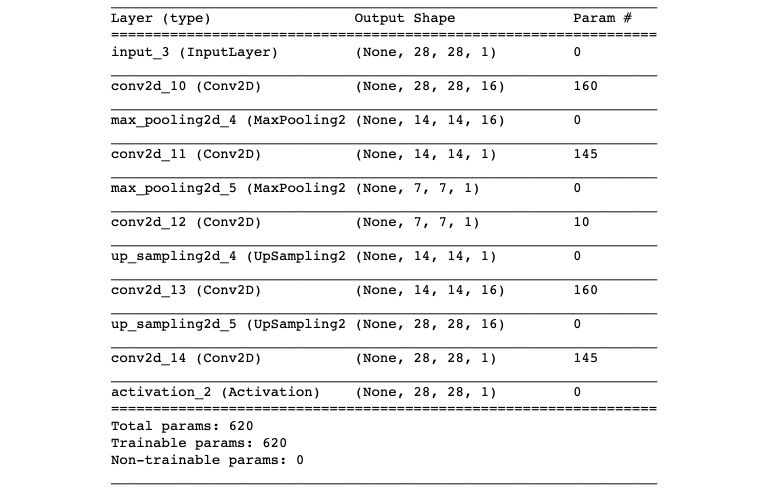
Using the hidden layers, we send the input image into a much lowe dimension :

` 771 = 49 `

Instead of :

` 28281 = 784 `

Now, let’s train the model! We don’t need any y_train here, both the input and the output will be the train images.

autoencoder.fit(X_train, X_train, nb_epoch = 15, batch_size = 64, validation_split = 0.1)

Save the weights of the autoencoder :

# Save autoencoder weight
json_string = autoencoder.to_json()
autoencoder.save_weights('autoencoder.h5')
open('autoencoder.h5', 'w').write(json_string)

We can build an encoding model using the first part of the model :

encoder = Model(inputs = input_img, outputs = encoded)

We can get the encoded input with :

X_train_enc = encoder.predict(X_train)

Visualize the output

We can simply visualize the output using the predict function of the autoencoding model :

encoded_imgs = encoder.predict(X_test)
decoded_imgs = autoencoder.predict(X_test)

To display the images, we can simply plot the entry image and the decoded image :

n = 10  
plt.figure(figsize=(20, 4))

for i in range(n):
    # display original
    ax = plt.subplot(3, n, i + 1)
    plt.imshow(x_test[i].reshape(28, 28))
    plt.gray()
    ax.get_xaxis().set_visible(False)
    ax.get_yaxis().set_visible(False)

    # Encoded images
    ax = plt.subplot(3, n, i + 1 + n)
    plt.imshow(encoded_imgs[i].reshape(7, 7))
    plt.gray()
    ax.get_xaxis().set_visible(False)
    ax.get_yaxis().set_visible(False)
    
    # display reconstruction
    ax = plt.subplot(3, n, i + 1 + 2*n)
    plt.imshow(decoded_imgs[i].reshape(28, 28))
    plt.gray()
    ax.get_xaxis().set_visible(False)
    ax.get_yaxis().set_visible(False)

plt.show()

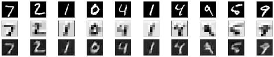
The first row is the input image. The middle row is the encoded image. The output row is the decoded image.

Our model remains quite simple, and we should add some epochs to reduce the noise of the reconstituted image.

Dense version

We have just made a deep convolutional autoencoder. Another version one could think of is to treat the input images as flat images and build the autoencoder using Dense layers.

input_img = Input(shape=(`shape_x * shape_y,))
encoded = Dense(128, activation='relu')(input_img)
encoded = Dense(64, activation='relu')(encoded)
encoded = Dense(32, activation='relu')(encoded)

decoded = Dense(64, activation='relu')(encoded)
decoded = Dense(128, activation='relu')(decoded)
decoded = Dense(shape_x * shape_y, activation='sigmoid')(decoded)

The Github repository of this article can be found here.

**Conclusion **: I hope this quick introduction to autoencoder was clear. Don’t hesitate to drop a comment if you have any question.

Maël Fabien

What is an autoencoder?

Variations

Create an autoencoder in Python

Visualize the output

Dense version