
You might have already heard of Fairseq, a sequence-to-sequence toolkit written in PyTorch by FacebookAI. One of the most common applications of Fairseq among speech processing enthusiasts is wav2vec (and all the variants), a framework that aims to extract new types of input vectors for acoustic models from raw audio, using pre-training and self-supervised learning.
In this article, we will cover the 4 core papers of this wav2vec series, all of them coming from Facebook AI. All these papers are building blocks of what could be a great innovation in speech recognition but also a lot of other downstream tasks related to speech:
- wav2vec paper
- vq - wav2vec
- wav2vec2.0 paper
- Self-training and Pre-training are Complementary for Speech Recognition
1. wav2vec
It is not new that speech recognition tasks require huge amounts of data, commonly hundreds of hours of labeled speech. Pre-training of neural networks has proven to be a great way to overcome limited amount of data on a new task.
a. What is pre-training?
What we mean by pre-training is the fact of training a first neural network on a task where lots of data are available, saving the weights, and creating a second neural network by initializing the weights as the ones saved from the first one. This learns general representations on huge amounts of data, and can supposedly improve the performance on the new task with limited data. This has been applied extensively in Computer Vision, Natural Language Processing, and more recently, for certain speech tasks.
When pre-training, you can either do it:
- in a supervised fashion
- or in an unsupervised fashion
Supervised pre-training is clear. This is similar to transfer learning where you pre-train a model, knowing you \(X\) and \(y\). But for unsupervised pre-training, you learn a representation of speech. wav2vec, is a convolutional neural network (CNN) that takes raw audio as input and computes a general representation that can be input to a speech recognition system. The objective is a contrastive loss that requires distinguishing a true future audio sample from negatives.
b. The model
Given an input signal context (speech up to a certain time-stamp), the aim is to predict the next observations from this speech sample.
Problem: This usually requires being able to properly model \(p(x)\), the distribution of speech samples.
Solution: Lower the dimensionality of the speech sample through an “encoder network”, and then use a context network to predict the next values. wav2vec learns representations of audio data by solving a self-supervised context-prediction task.
More formally, given audio samples \(x_i \in X\), we:
- learn a first encoder network, based on a CNN, that maps \(X\) to \(Z\):
- learn a second context network, based on a CNN too, that maps \(Z\) to a single contextualized tensor \(C\):
A representation of these 2 networks is presented in the figure below:
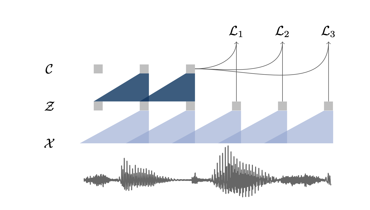
Here are the network details of wav2vec implementation:
- the encoder is a 5-layer CNN, with kernel sizes (10, 8, 4, 4, 4) and strides (5, 4, 2, 2, 2), and covers 30ms of audio. Layers have 512 channels, a group normalization layer, and a ReLU nonlinearity.
- the context network has nine layers with kernel size three and stride one, and the total receptive field of the context network is about 210 ms. Layers have 512 channels, a group normalization layer, and a ReLU nonlinearity.
c. Loss function
The model learns to distinguish a true sample \(z_{ik}\), \(k\) steps in the future, from a proposal distribution \(p_n\), called a contrastive loss, defined by:
\[\mathcal{L}_{k}=-\sum_{i=1}^{T-k}\left(\log \sigma\left(\mathbf{z}_{i+k}^{\top} h_{k}\left(\mathbf{c}_{i}\right)\right)+\underset{\tilde{\mathbf{z}} \sim p_{n}}{\mathbb{E}}\left[\log \sigma\left(-\mathbf{\tilde { z }}^{\top} h_{k}\left(\mathbf{c}_{i}\right)\right)\right]\right)\]We then optimize the loss over several time steps:
\[\mathcal{L} = \sum_{k=1}^K \mathcal{L}_k\]To get the expectation of the proposal distribution, we sample ten negative examples by choosing uniformly distractors from these negative audio sequences. In order words, we average ten uniformly sampled values from different audio samples. \(\lambda\) is the number of negative samples (10 lead to the best performance).
By predicting the next steps, we perform a task, called self-supervised training for speech. But it is also widely applied in NLP and CV.
d. Self-supervised learning
In self-supervised learning, we train a model using labels that are naturally part of the input data, rather than requiring separate external labels. For example, in an NLP model, we train a model to predict the next words. This information is part of the training data itself, and the model learns some information on the nature of language. Think of models like GPT or ULMFiT that do this in NLP. GPT-3 appears to be so good at this that you can use it for Question Answering on generic topics without fine-tuning, and get proper replies.
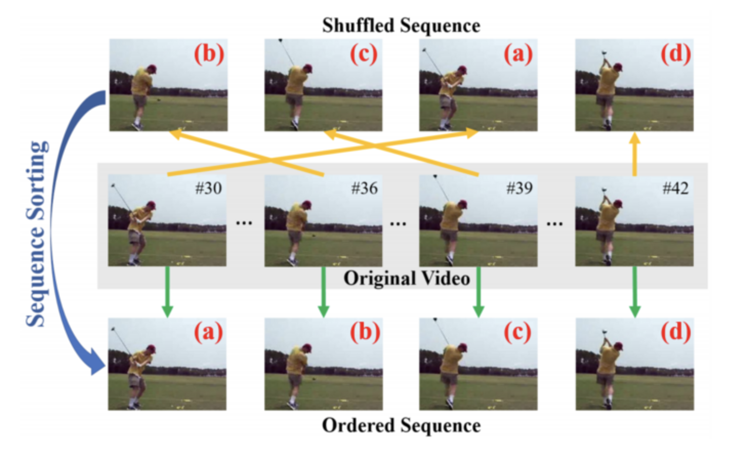
In Computer Vision, the implementation is slightly different. We still need to train a model in a self-supervised way using a “context task”, with the idea to focus on a “downstream task”. Several pretext tasks can be used, such as colorization, placing images in patches, placing frames in the right order… For videos, for example, a common workflow is to train a model on one or multiple pretext tasks with unlabelled videos and then feed one intermediate feature layer of this model to fine-tune a simple model on downstream tasks of action classification, segmentation, or object tracking.
Self-supervised training can allow you to use 1000x less training data for a given downstream task.
e. Acoustic Models
wav2vec is used as an input to an acoustic model. The vector supposedly carries more representation information than other types of features. It can be used as an input in a phoneme or grapheme-based wav2letter ASR model. The model then predicts the probabilities over 39-dimensional phoneme or 31-dimensional graphemes.
f. Decoding
Regarding the language model decoding, the authors considered a 4-gram language model, a word-based convolutional language model, and a character-based convolutional language model. Word sequences are decoded using beam-search.
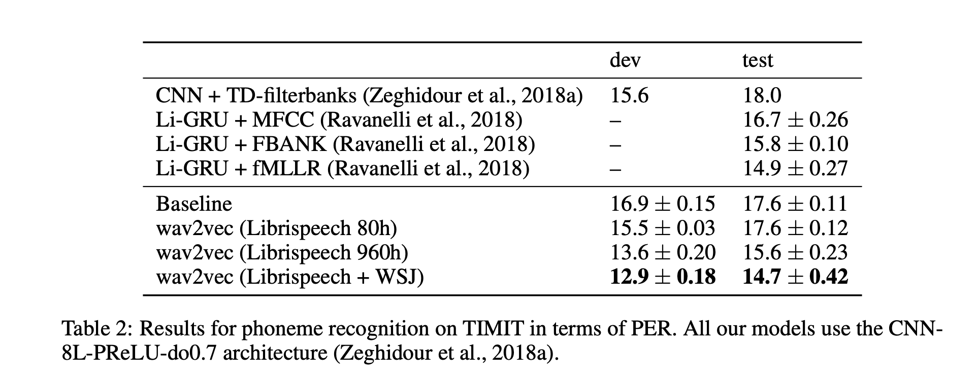
g. Results
Pre-training reduces WER by 36 % on nov92 when only about eight hours of transcribed data is available. It also improved the PER on the TIMIT database compared to a baseline system, and the more pre-training data, the better the results were (Librispeech + WSJ in their best system). Results on TIMIT are presented in the table below.
2. vq-wav2vec
vq-wav2vec introduces self-supervised learning of discrete speech representations. What we mean by discrete here is that we do not have vectors that take continuous values, but a set of given values only. Discretization, rather than enables the direct application of algorithms from the NLP community which require discrete inputs. In other words, vq-wav2vec, learns vector quantized (VQ) representations of audio data using a future time-step prediction task.
a. Model architecture
The model is said to word on discrete speech representations since it adds an additional layer of quantization.
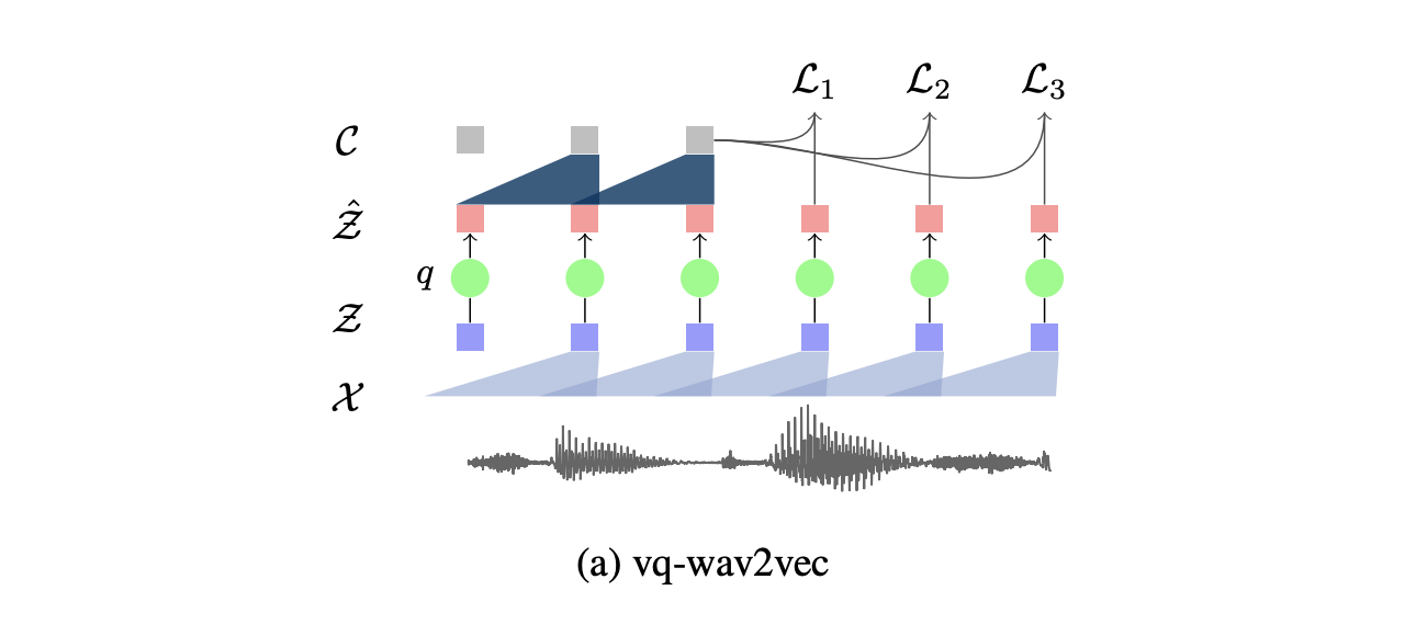
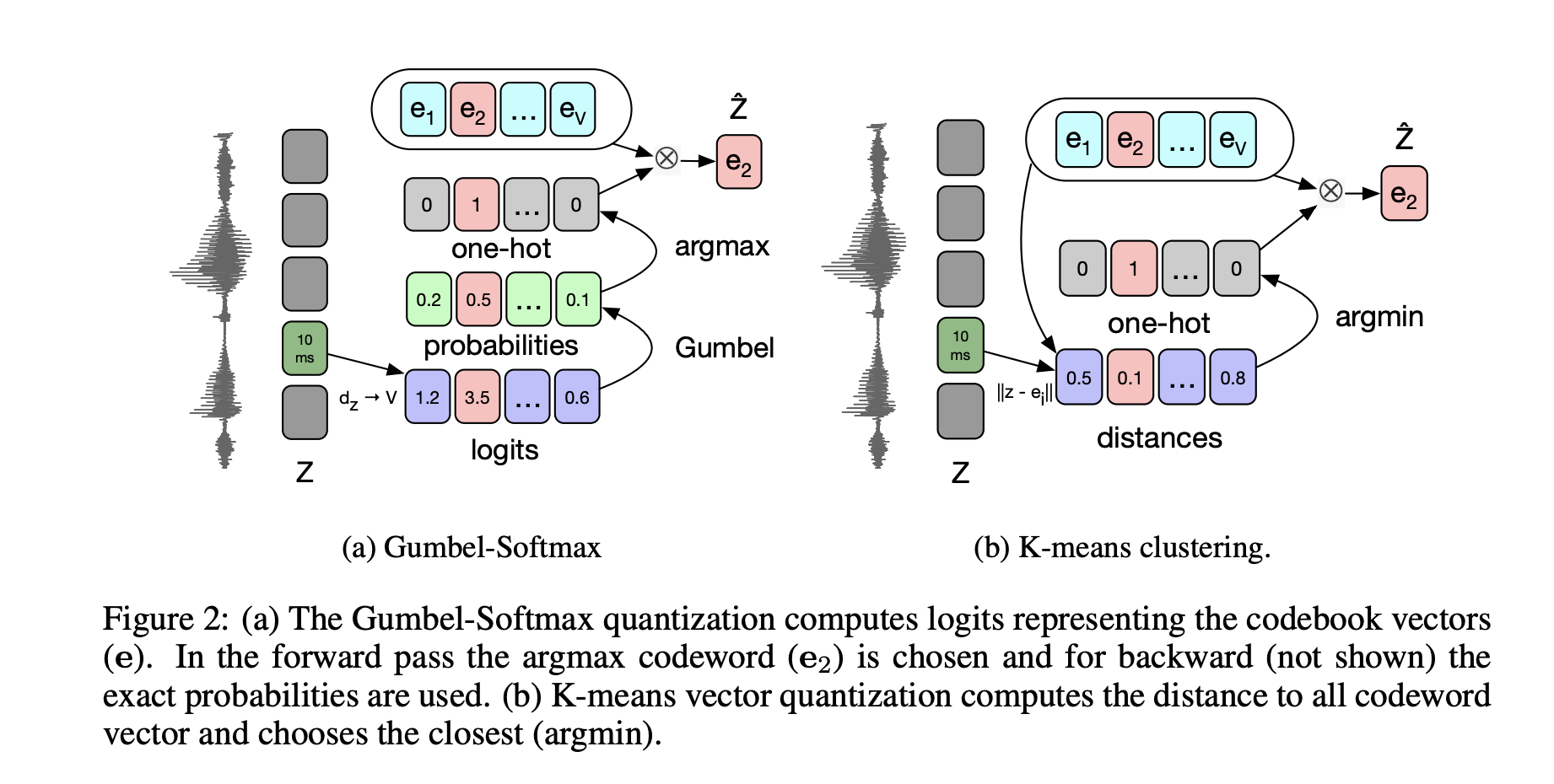
This additional layer \(q : Z \to \tilde{Z}\) that takes \(Z\), a dense representation learned by the first CNN, and outputs a discrete representation, using either K-means clustering or the Gumbel-Softmax as constraints in a Vector Quantized Variational Autoencoders.
Finally, this discrete representation is fed as an input to the context network \(g : \tilde{Z} \to C\).
b. What to do with this discrete representation?
The discrete speech representation is then fed to train a BERT architecture. BERT is a pre-training approach for NLP tasks, which uses a transformer encoder model to build a representation of text. Transformers use self-attention to encode the input sequence as well as an optional source sequence.
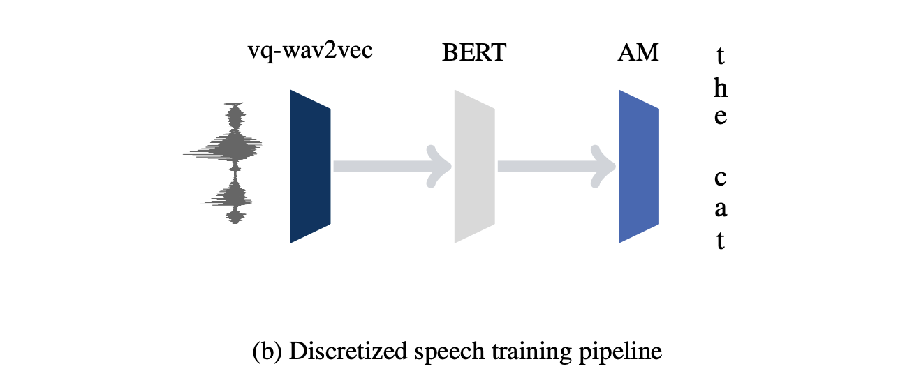
In prediction, we fetch speech representations that are used as inputs to an acoustic model.
c. Acoustic Model
Authors used wav2letter as an acoustic model and trained for 1,000 epochs on 8 GPUs for both TIMIT and WSJ. Language models used were a 4-gram KenLM language model and a character-based convolutional language model.
d. Results
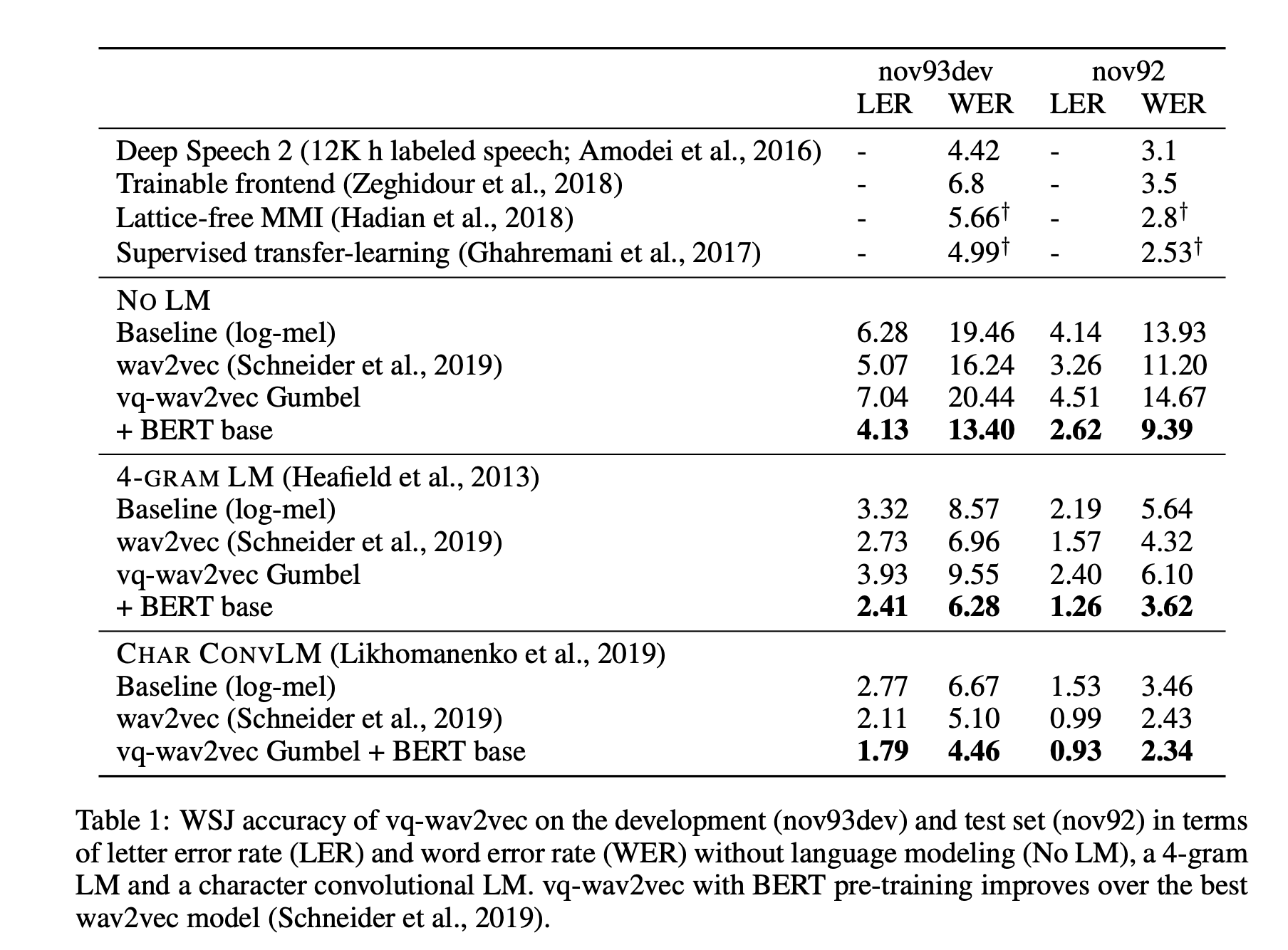
Results on the character-based convolution language model and a Gumbel + Bert base vq-wav2vec reach state-of-the-art on the WSJ dataset.
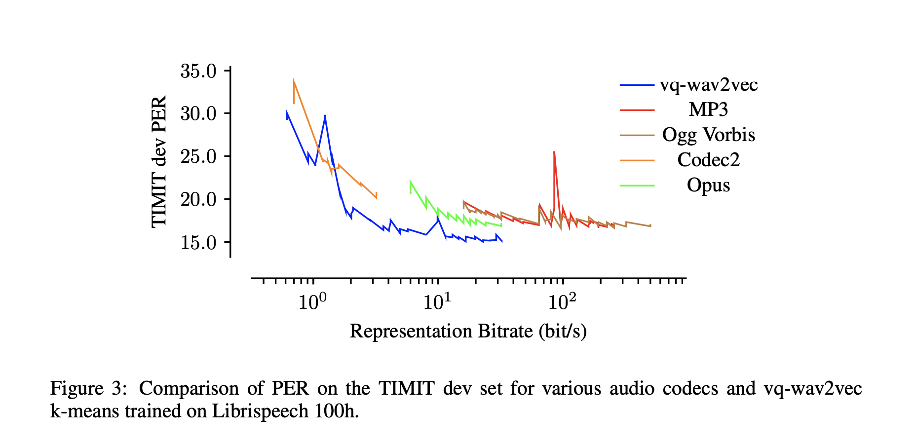
Another important contribution of this paper is that, by exploring quantization, highly reduces the bitrate for a given model performance. Acoustic models on vq-wav2vec achieve the best results across most bitrate settings.
e. End-to-end model
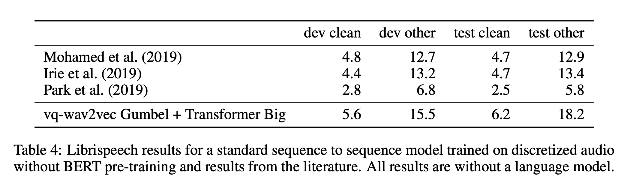
One last important work, although results were not that good, is the sequence-to-sequence model that authors explain in a small paragraph. Rather than training BERT on discretized speech, and inputting it in the acoustic model, one could solve speech recognition as an end-to-end task.
This is solved by taking the discrete speech representation as an input to a Transformer architecture. Hence, no acoustic model is required. No language model or data augmentation was used, which might explain the limited results. But this work is an important step towards what the next papers of this series explore.
3. wav2vec 2.0
wav2vec 2.0 leverages self-supervised training, like vq-wav2vec, but in a continuous framework from raw audio data. It builds context representations over continuous speech representations and self-attention captures dependencies over the entire sequence of latent representations end-to-end.
a. Model architecture
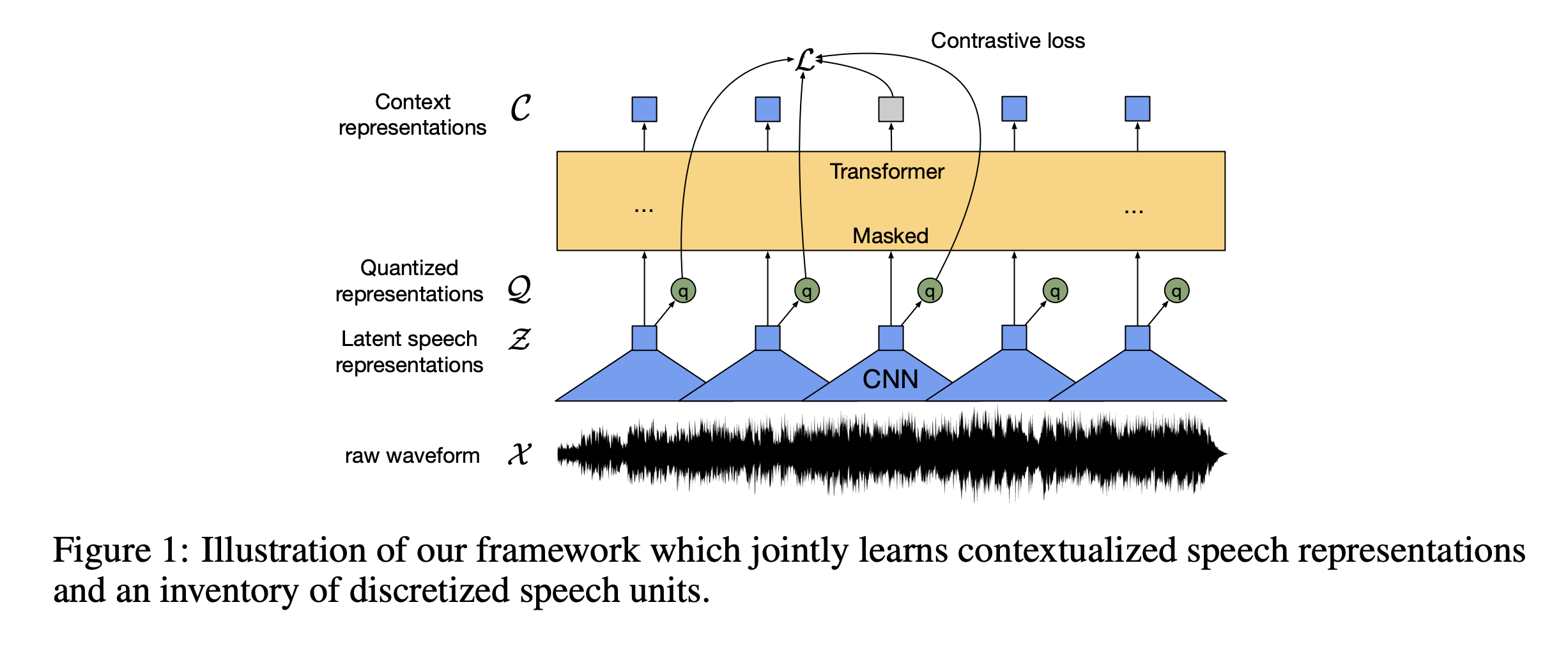
Inspired by the end-to-end version of the vq-wav2vec paper, the authors further explored this idea with a novel model architecture:
- the feature encoder, made of several blocks of temporal convolution followed by layer normalization and a GELU activation function, learns a latent representation: \(f : X \to Z\). Part of the output of this layer is masked before being used as an input to the context network.
- the output of the feature encoder is fed to a context network that follows the Transformer architecture and uses convolutional layers to learn relative positional embedding. \(g : Z \to C\)
- the output of the feature encoder (and not of the context transformer) is discretized in parallel using a quantization module that relies on product quantization. Product quantization amounts to choosing quantized representations from multiple codebooks and concatenating them, which is then used as an input to a Gumbel softmax to select the quantized representations.
The model architecture is summarized below:
b. Loss function
As you might have seen, the loss depends on 2 components:
- a contrastive loss \(L_m\), where the model needs to identify the true quantized latent speech representation, and distractors. Distractors are uniformly sampled from other masked time steps of the same utterance.
- a diversity loss \(L_d\) to encourage the model to use the codebook entries equally often
The overall loss is defined by :
\[L = L_m + \alpha L_d\]c. Fine-tuning for downstream speech recognition task
The authors added a randomly initialized linear projection on top of the context network (transformer) into \(C\) classes representing the vocabulary of the task. For Librispeech, we have 29 tokens for character targets plus a word boundary token. Models are optimized by minimizing a CTC loss.
d. Language models
2 types of language models were considered:
- a 4-gram model
- and a transformer trained on Librispeech
Beam search decoding was used.
e. Results
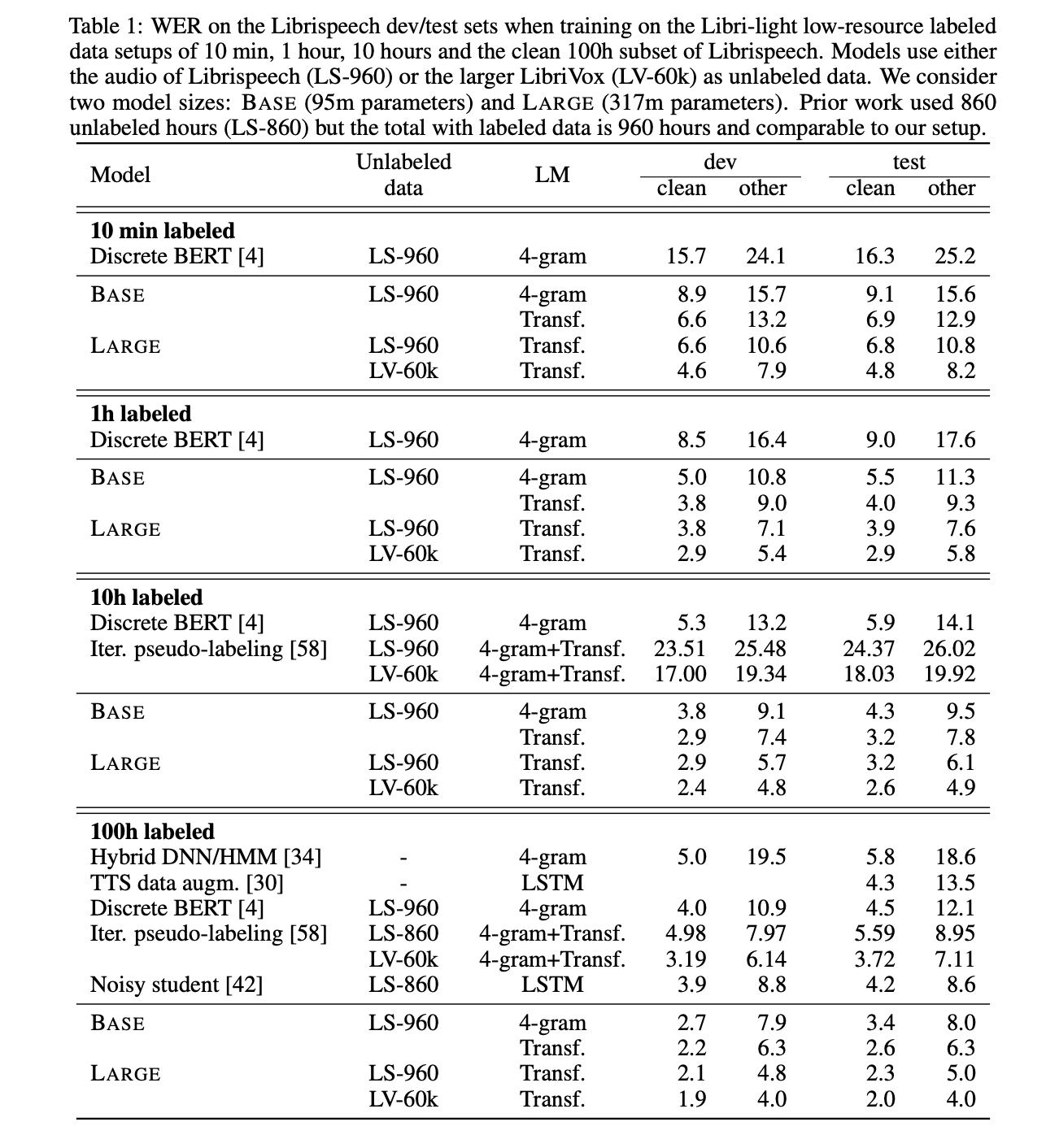
If a pre-trained model captures the structure of speech, then it should require few labeled examples to fine-tune it for speech recognition.
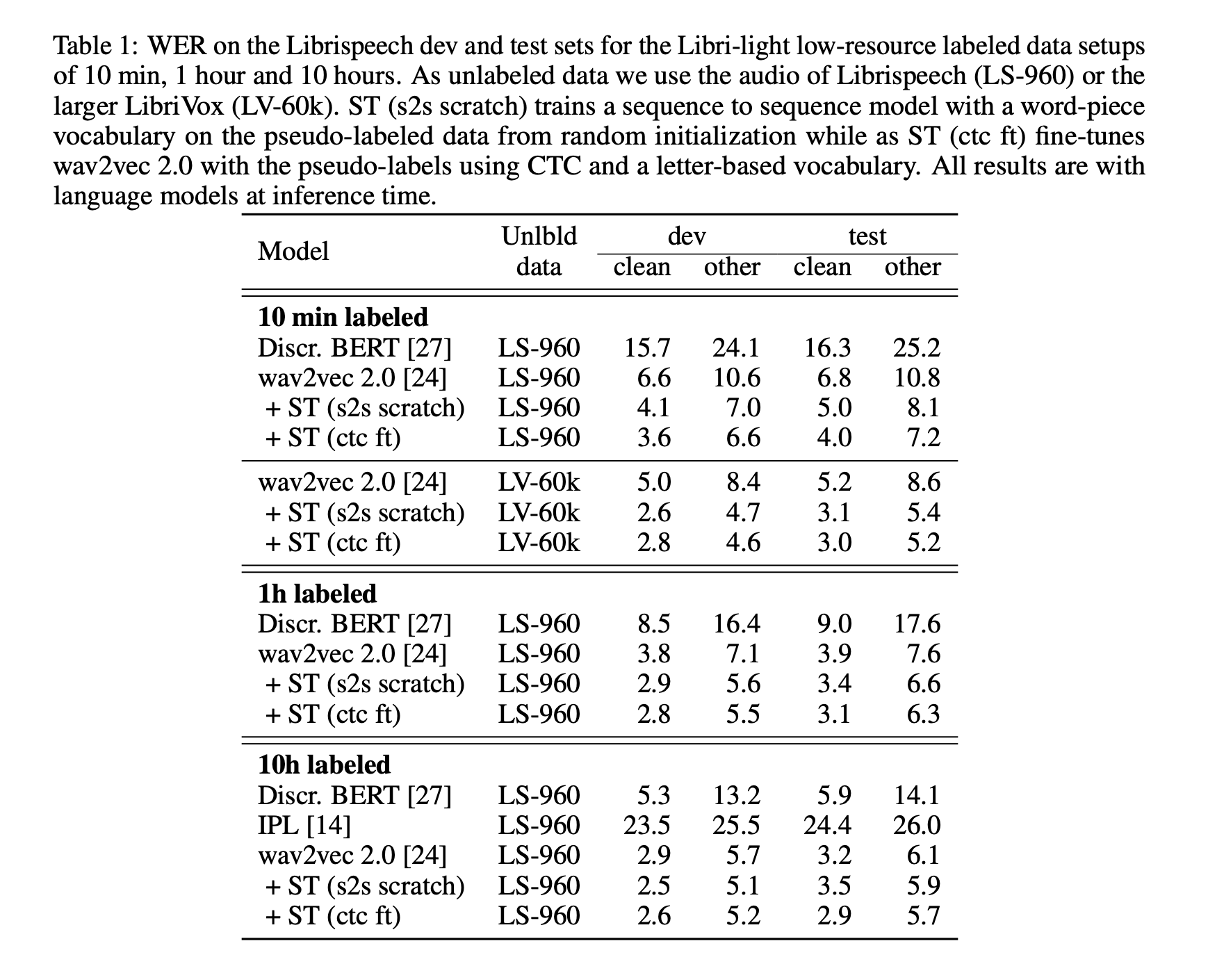
The LARGE model pre-trained on LibriVox (LV-60k) and fine-tuned on only 10 minutes of labeled data achieves a word error rate of 5.2/8.6 on the Librispeech clean/other test sets. This is definitely a major milestone in speech recognition for ultra-low resource language. This demonstrates that ultra-low resource speech recognition is possible with self-supervised learning on unlabeled data
Of course, the more labeled data is processed for fine-tuning, the better the model performance.
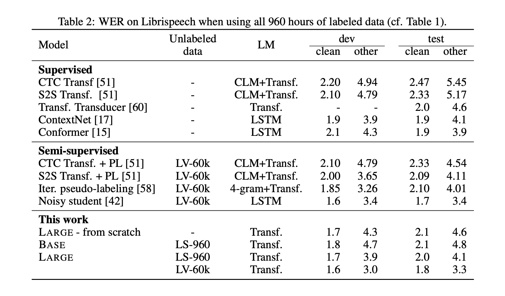
But what happens when lots of training data are available? Does it beat SOTA?
The ten-minute models without lexicon and language model tend to spell words phonetically and omit repeated letters, e.g., will → wil. Spelling errors decrease with more labeled data.
When even more training data are available, e.g. the whole of Librispeech, the architecture reaches SOTA results.
Finally, the authors mention that self-training is likely complimentary to pre-training and their combination may yield even better results. However, it is not clear whether they learn similar patterns or if they can be effectively combined.
4. Self-training and Pre-training are Complementary for Speech Recognition
This last work combines both self-supervised training and pre-training for speech recognition. It gained a lot of attention lately, especially on Twitter with this headline that just 10 minutes of labeled speech can reach the same WER than a recent system trained on 960 hours of data, from just a year ago.
Great progress in speech recognition: wav2vec 2.0 pre-training + self-training with just 10 minutes of labeled data rivals the best published systems trained on 960 hours of labeled data from just a year ago.
— Michael Auli (@MichaelAuli) October 26, 2020
Paper: https://t.co/niBzDiei1j
Models: https://t.co/frCK1GJMZQ pic.twitter.com/AjEWdna6J1
In their paper, the authors explore the complementarity of self-training and pre-training.
The pre-training approach adopted so far relied on self-supervised learning. This whole block will now be referred to as unsupervised pre-training. This paper introduces the notion of self-training.
a. Self-training
In self-training, we train an initial acoustic model on the available labeled data and then label the unlabeled data with the initial model as well as a language model in a step we call pseudo-labeling. Finally, a new acoustic model is trained on the pseudo-labeled data as well as the original labeled data.
Self-training and pre-training are then mixed in the following way:
- first, pre-train a wav2vec 2.0 model on the unlabeled data (using self-supervised learning approach),
- fine-tune it on the available labeled data in an end-to-end fashion using CTC loss and a letter-based output vocabulary,
- then use the model to label the unlabeled data using self-training
- and finally, use the pseudo-labeled data to train the final model.
For the self-training part,
- first, generate a list of candidate transcriptions by combining wav2vec 2.0 and the standard Librispeech 4-gram language model during beam-search
- the n-best list is pruned to the 50 highest scoring entries and then rescored with a Transformer LM trained on the Librispeech language corpus
The final model trains a Transformer-based sequence to sequence model with log-Mel filterbank inputs after pseudo-labeling using wav2letter++. It uses a 10k word piece output vocabulary computed from the training transcriptions if the whole Librispeech training set is used as labeled data.
b. Results
Results achieved on only 10 minutes of data are even better than wav2vec 2.0.
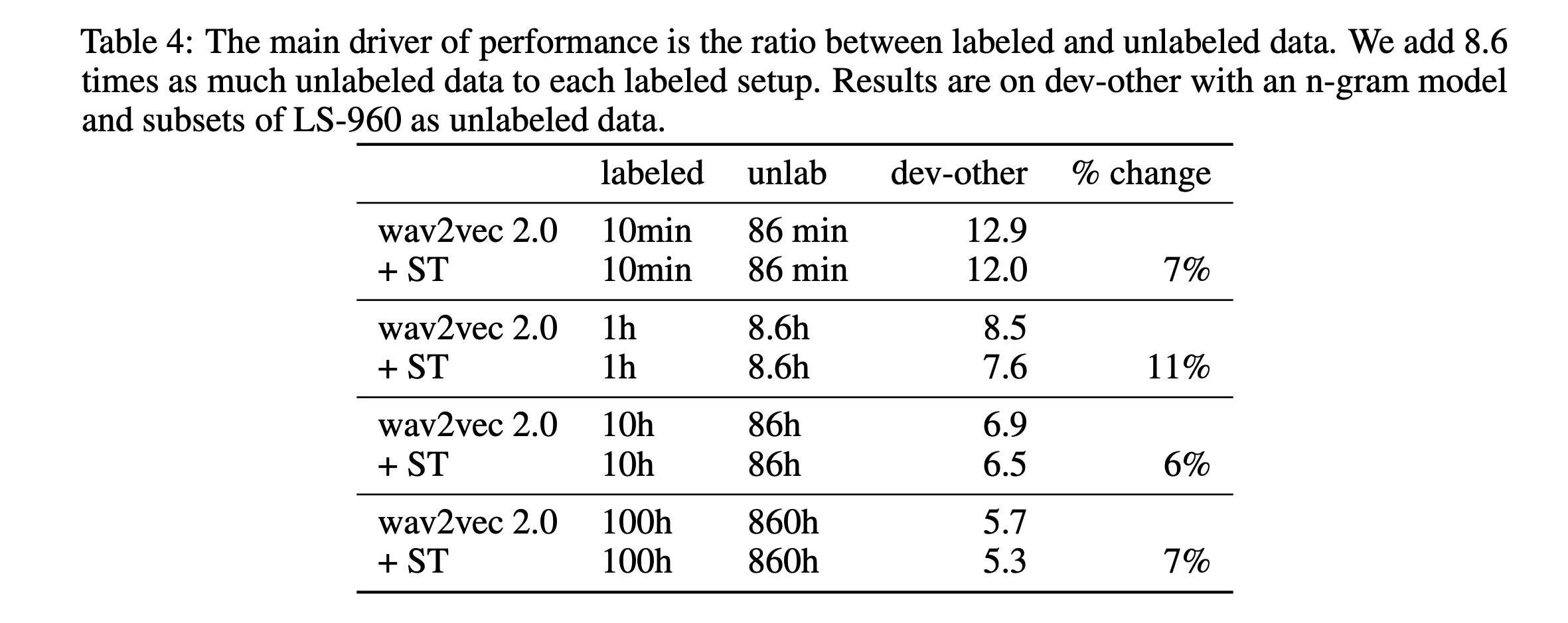
Finally, the authors explore to what extent self-training and pre-training are complementary. According to the table below, it appears when respecting a ratio of 8.6 times more unlabeled speech that labeled one, self-training keeps improving results by more than 7% on average.
5. The code!
Luckily, Patrick Von Platen, research engineer at Hugging Face, let a comment below, and guess what… Wav2Vec2 is in Hugging Face Transformer’s library!
Here is the link to the PR. And if you want to have access to a Wav2Vec2 model, pre-trained on LibriSpeech, it’s as easy as:
pip install git+https://github.com/huggingface/transformers
And then:
import librosa
import soundfile as sf
import torch
from transformers import Wav2Vec2ForCTC, Wav2Vec2Tokenizer
import nltk

def load_model():
    tokenizer = Wav2Vec2Tokenizer.from_pretrained("facebook/wav2vec2-base-960h")
    model = Wav2Vec2ForCTC.from_pretrained("facebook/wav2vec2-base-960h")
    return tokenizer, model

def correct_sentence(input_text):
    sentences = nltk.sent_tokenize(input_text)
    return (' '.join([s.replace(s[0],s[0].capitalize(),1) for s in sentences]))

def asr_transcript(input_file):

    tokenizer, model = load_model()

    speech, fs = sf.read(input_file)

    if len(speech.shape) > 1:
        speech = speech[:,0] + speech[:,1]

    if fs != 16000:
        speech = librosa.resample(speech, fs, 16000)

    input_values = tokenizer(speech, return_tensors="pt").input_values
    logits = model(input_values).logits

    predicted_ids = torch.argmax(logits, dim=-1)

    transcription = tokenizer.decode(predicted_ids[0])

    return correct_sentence(transcription.lower())
Thanks a lot to Hugging Face for such an easy implementation. Next features will probably include training of such models, and that’s an exciting move towards speech for Hugging Face!
6. Conclusion
a. Brief summary
We have seen in this article:
- that wav2vec can be used as a new representation of speech, which can itself be used as inputs to other downstream tasks such as speech recognition
- that for ASR, wav2vec, i.e. pre-training using self-supervised learning on a large amount of unlabeled data can help the model performance on a limited amount of data later
- that end-to-end models with CTC loss using wav2vec 2.0 inputs work well
- that self-training and pre-training appear to be complementary
- that 10 minutes of labeled speech might be sufficient to train a good ASR system
initial self-supervised learning
b. What is really embedded in this speech representation?
Well, this is an open research question. I am really interested in exploring this. This is what I have currently found:
- wav2vec embeds language id information, which can be then used for language classification: Comparison of Deep Learning Methods for Spoken Language Identification
- wav2vec, in a modified version, might directly contain information related to speakers, and could therefore be used for speaker verification tasks, or fused with X-vectors: Wav2Spk: A Simple DNN Architecture for Learning Speaker Embeddings from Waveforms
Speech representations can be used for several downstream tasks. I am rather convinced that it is a matter of time before these representations, learned from raw waveforms, approach SOTA or even beat it on other tasks such as speaker identification, voice activity detection, language identification, pathological speech detection… I see it as a very powerful tool.
Final word
I hope this wav2vec series summary was useful. Feel free to leave a comment
All references: