
So far, we considered the HMM training under the Maximum Likelihood Estimate (MLE). But the MLE is only optimal under certain model correctness assumptions: Observations should be conditionally independent given the hidden state, which is not the case if states are phone based for example.
Recall: MLE of HMMs
The MLE identifies the best set of parameters to maximize the objective function:
\[F_{MLE} = \sum_{u=1}^U \log P_{\lambda}(X_u \mid M(W_u))\]Where:
- \(X_u\) are the training utterances
- \(W_u\) are the word sequences
- \(M(W_u)\) are the corresponding HMM to the word sequences
- \(\lambda\) is the set of parameters of the HMM
Then, in an HMM-GMM for example, we define the mean vector \(\mu_{jm}\) for the mth Gaussian component in the jth state as:
\[\hat{\mu_{jm}} = \frac{\sum_u \sum_t \gamma_{jm}^u(t) x_t^u}{\sum_u \sum_t \gamma_{jm}^u(t)}\]Where \(\gamma_{jm}^u(t)\) is the probability of being in mixture m at state j at time t given training sentence u.
Before introducing discriminative training, let us introduce 2 additional pieces of notation:
\[\Theta_{jm}^u(M) = \sum_t \gamma_{jm}^u(t) x_t^u\] \[\Gamma_{jm}^u(M) = \sum_t \gamma_{jm}^u(t)\]Therefore, we can re-write the mean vector as:
\[\hat{\mu_{jm}} = \frac{\sum_u \Theta_{jm}^u(M(W_u)) }{\sum_u \Gamma_{jm}^u(M(W_u)) }\]Maximum mutual information estimation (MMIE)
This sections applies for HMM-GMM architectures.
The MMIE aims to directly maximize the posterior probability.
\[F_{MMIE} = \sum_u \log P_{\lambda}(M(W_u) \mid X_u)\]We can then decompose it into an acoustic and a language model:
\[F_{\mathrm{MMIE}}=\sum_{u=1}^{U} \log \frac{P_{\lambda}\left(\mathbf{X}_{u} \mid M\left(W_{u}\right)\right) P\left(W_{u}\right)}{\sum_{W^{\prime}} P_{\lambda}\left(\mathbf{X}_{u} \mid M\left(W^{\prime}\right)\right) P\left(W^{\prime}\right)}\]What this ratio represents is the likelihood of data given correct word sequence divided by the total likelihood of data given all possible word sequences.
We optimise \(F_{MMIE}\) by making the correct word sequence likely (numerator goes up), and the other word sequences unlikely (denominators goes down).
The optimization is done using an Extended Baum-Welch algorithm (EBW), and the new mean update equation is given by:
\[\hat{\mu}_{j m}=\frac{\sum_{u=1}^{U}\left[\Theta_{j m}^{u}\left(\mathcal{M}_{\mathrm{num}}\right)-\Theta_{j m}^{u}\left(\mathcal{M}_{\mathrm{den}}\right)\right]+D \mu_{j m}}{\sum_{u=1}^{U}\left[\Gamma_{j m}^{u}\left(\mathcal{M}_{\mathrm{num}}\right)-\Gamma_{j m}^{u}\left(\mathcal{M}_{\mathrm{den}}\right)\right]+D}\]Lattice-based sequence training
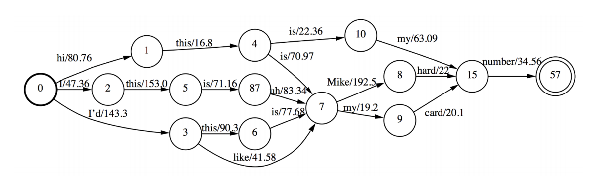
To compute the denominator in the \(F_{MMIE}\), we must sum over all possible word sequences, which is hard. The idea of using lattices is to estimate the denominator by generating word lattices and summing over all words in the lattice. This way, we approximate the sum by a set of likely word sequences determined via a decoding run on the training data.
A word lattice is a directed acyclic graph with a single start point and edges labeled with a word and weight. It’s usually represented as a WFSTs, and allow you to only explore possible paths for word sequences rather than all combinations. Pruning in that WFST is also possible.
Minimum Phone Error (MPE)
We can also adjust the optimization criterion so that it’s directly related to the Word Error Rate in a method called Minimum Phone Error.
The new criterion becomes:
\[F_{\mathrm{MPE}}=\sum_{u=1}^{U} \log \frac{\sum_{W} P_{\lambda}\left(\mathbf{X}_{u} \mid \mathcal{M}(W)\right) P(W) A\left(W, W_{u}\right)}{\sum_{W^{\prime}} P_{\lambda}\left(\mathbf{X}_{u} \mid \mathcal{M}\left(W^{\prime}\right)\right) P\left(W^{\prime}\right)}\]Where \(A(W, W_u)\) is the phone transcription accuracy of the sentence \(W\) given reference \(W_u\).
It’s a weighted average over all possible sentences \(w\) of the raw phone accuracy, and finds probable sentences with low phone error rates.
Discriminative training of DNNs
So far, we saw what could be applied for HMM-GMM architectures. DNNs are trained in a discriminative manner, since the cross entropy (CE) with a softmax pushes the correct label and pulls down the competing labels. But can we train DNN systems with an MMI objective function?
Yes, we can, and this is usually done the following way:
- train a DNN system framewise using cross-entropy (CE)
- use the trained model to generate alignments and lattices for sequence training
- use the trained weights to initialize the weights for sequence training
- train a new DNN system and use back-propagation with sequence training objective function (e.g. MMI)
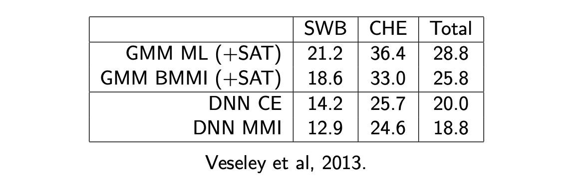
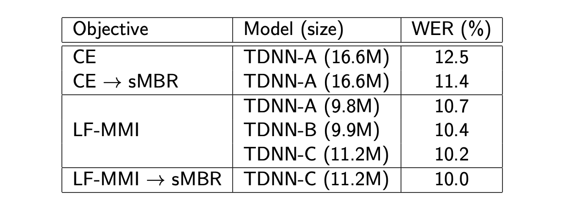
The results of various approaches on the Switchboard dataset are presented below:
Lattice-Free MMI (LF-MMI)
The aim of Lattice-Free MMI is to avoid the need to pre-compute lattices for the denominator, and the need to train using frame-based Cross Entropy before sequence training.
Lattice-free MMI is basically made of a few tips:
- both numerator and denominator are represented as HCLG FSTs
- denominator forward-backward computation is parallelized on GPU
- the word-level LM is replaces with a 4-gram phone LM
- frame rate is reduced at 30ms
- train on small fixed-size chunks (1.5 seconds)
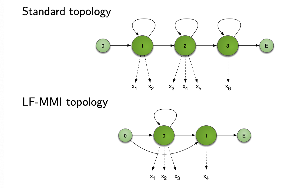
- HMM topology is simpler, and can be traversed in a single frame, called leaky HMM
Regularisation is also used, by using standard CE objective as a secondary task. All layers but the final are then shared between tasks.
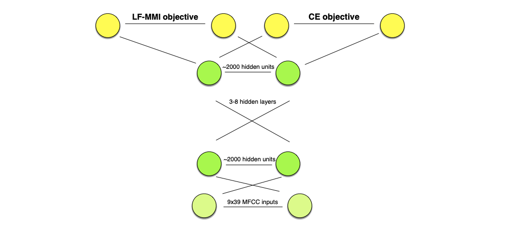
We also apply L2 regularisation on the main output.
LF-MMI is faster to train and decode and achieves better WER. It however performs worse when training transcripts are unreliable.
As a summary, we usually intialise sequence discriminative training:
- HMM/GMM – first train using ML, followed by MMI
- HMM/NN – first train at frame level (CE), followed by MMI
But LF-MMI seems to bring current SOTA and lower computational costs.
Conclusion
If you want to improve this article or have a question, feel free to leave a comment below :)
References: