
When training an ASR system, mismatch can occur between training and test data, due to various sources of variation. Speaker adaptation can help fill this gap.
Sources of variation
Acoustic model
Lots of speaker-specific variations exist in the acoustic model:
- speaking styles
- accents
- speech poduction anatomy
There are also variations not related to the speaker itself, but to the channel (telephone, distance to microphone, reverberation…).
Pronunciation model
Each speaker has a specific way to pronounce some words.
Language model
Test data might be related to a specific topic, or to user-specific documents. The language model should then be adapted.
To handle all of these potential variations, we perform speaker adaptation. The aim is to reduce the mismatch between test data and trained models.
ASR Systems can be said to be:
- Speaker Independent (SI), which does not require too much data for each speaker, but has high WER
- Speaker Dependent (SD), which requires a lot of data per speaker
- Speaker Adaptative, that builds on top of an SI system and requires only a fraction of speaker-specific training data from an SD system
Speaker Adaptation (SA)
Adaptation can be:
- supervised, if word level transcriptions of adaptation data is known
- unsupervised, if no transcripts are available
It can also be:
- static, if we adapt on adaptation data in a block
- dynamic, if we adapt incrementally
Finally, we want SA to be:
- compact, few speaker-dependent parameters
- efficient, requires low computational resources
- flexible, applicable to different models
Model-based adaptation
We can adapt the parameters of acoustic models to better match the observed data, using:
- Maximum A Posteriori (MAP) adaptation of HMM/GMM
- Maximum Likelihood Linear Regression (MLLR) of GMMs, and cMLLR
- Learning Hidden Unit Contributions (LHUC) for NNs
Adaptation of HMM-GMMs
MAP training of GMMs
MAP training will balance the estimated parameters of the Speaker Independent data and the new adaptation data.
Using Maximum Likelihood Estimate (MLE) os Speaker Independent model, the mth Gaussian in the jth state has the following mean:
\[\mu_{mj} = \frac{\sum_n \gamma_{jm}(n) x_n}{\sum_n \gamma_{jm}(n)}\]Where \(\gamma_{jm}\) is the component occupation probability. The aim of a MLE is to maximize: \(P(X \mid \lambda)\) where \(\lambda\) are the model parameters.
The MAP estimate of the adapted model uses the Speaker Independent models as a prior probability distribution over model parameters to estimate speaker-specific data. MAP training maximizes: \(P(\lambda \mid X) ∝ P(X \mid \lambda) P_0(\lambda)\)
It gives a new mean:
\[\hat{\mu} = \frac{ \tau \mu_0 + \sum_n \gamma(n)x_n} {\tau + \sum_n \gamma(n)}\]Where:
- \(\tau\) is a weight factor for the weight of the SI estimate (between 0 and 20 typically)
- \(x_n\) is the adaptation vector at time \(n\)
- \(\gamma(n)\) is the probability of this Gaussian at this time
- \(\mu_0\) is the prior mean
As the amount of training data increases, the MAP estimate converges to the ML one.
Maximum Likelihood Linear Regression (MLLR)
One of the issues with MAP is that with few adaptation data, most Gaussians will not be adapted. If instead we share the adaptation across the Gaussians, each adaptation data can affect many of, or all, the Gaussians.
As its name suggests, MLLR will apply a linear transformation on the Gaussian parameters estimated by MLE:
\[\hat{\mu} = A \mu + b\]Hence, if the observations have \(d\) -dimensions, then A is \(d \times d\) and b has \(d\) dimensions.
It can be re-written as:
\[\hat{\mu} = W \eta\]Where:
- \[W = [bA]\]
- \[\eta = [1 \mu^T]^T\]
We then estimate \(W\) to maximize the MLE on the adaptation data. Such transformations can then be applied to all classes, or to a set of Gaussian sharing a transform, called a regression class.
We must then determine the number of regression classes. This is usually small (1, 2 (speech / non-speech), one per broad class, one per context-independent phone class…). We can obtain the number of regression classes by building a regression class tree, in a similar manner to a clustering tree.
As usual in MLE, we maximize the log-likelihood (LL), which turns out to be easier to solve. The LL is defined as:
\[L = \sum_r \sum_n \gamms_r(n) \log (K_r \exp(-\frac{1}{2}(x_n - W \eta_r)^T \Sigma_r^{-1} (x_n - W \eta_r)))\]Where \(r\) defines the different regression classes. Note that there is bi closed form solution if \(\sigma\) is a full covariance matrix, and it can be solved if \(\sigma\) is diagonal.
We apply the mean-only MLLR, by adapting only the mean, and it usually improves WER by 10-15% (relative). 1 minute of adaptation speech is more or less equal, in terms of model performance, to 30 minutes of speech in speaker dependent models.
Constrained MLLR (cMLLR)
In constrained MLLR (cMLLR), we use the the same linear transform for both the mean and the covariance. This is also called feature space MLLR (fMLLR), since it’s equivalent to applying a linear transform to the data:
\[\hat{\mu} = A^{'} \mu - b^{'}\] \[\hat{\Sigma} = A^{'} \Sigma A^{'}^T\]There are no closed form solution, this is solved iteratively.
Speaker-Adaptative Training (SAT)
In SAT, we adapt the base models to the training speaker while training, using MLLR or fMLLR for each training speaker. It results in higher training likelihoods and improved recognition results, but increases the complexity and the storage requirements. SAT can be seen as a type of speaker normalization at training time.
Adaptation of HMM-DNNs
cMLLR feature transformation
We can use the HMM/GMM system that we train to estimate the tied state, to also estimate a single cMLLR transform for a given speaker. We then use this to transform the input speech of the DNN for the target speaker.
Linear Input Network (LIN)
In a Linear Input Network (LIN), a single linear input layer is trained to map input speaker-dependent speech to speaker independent network.
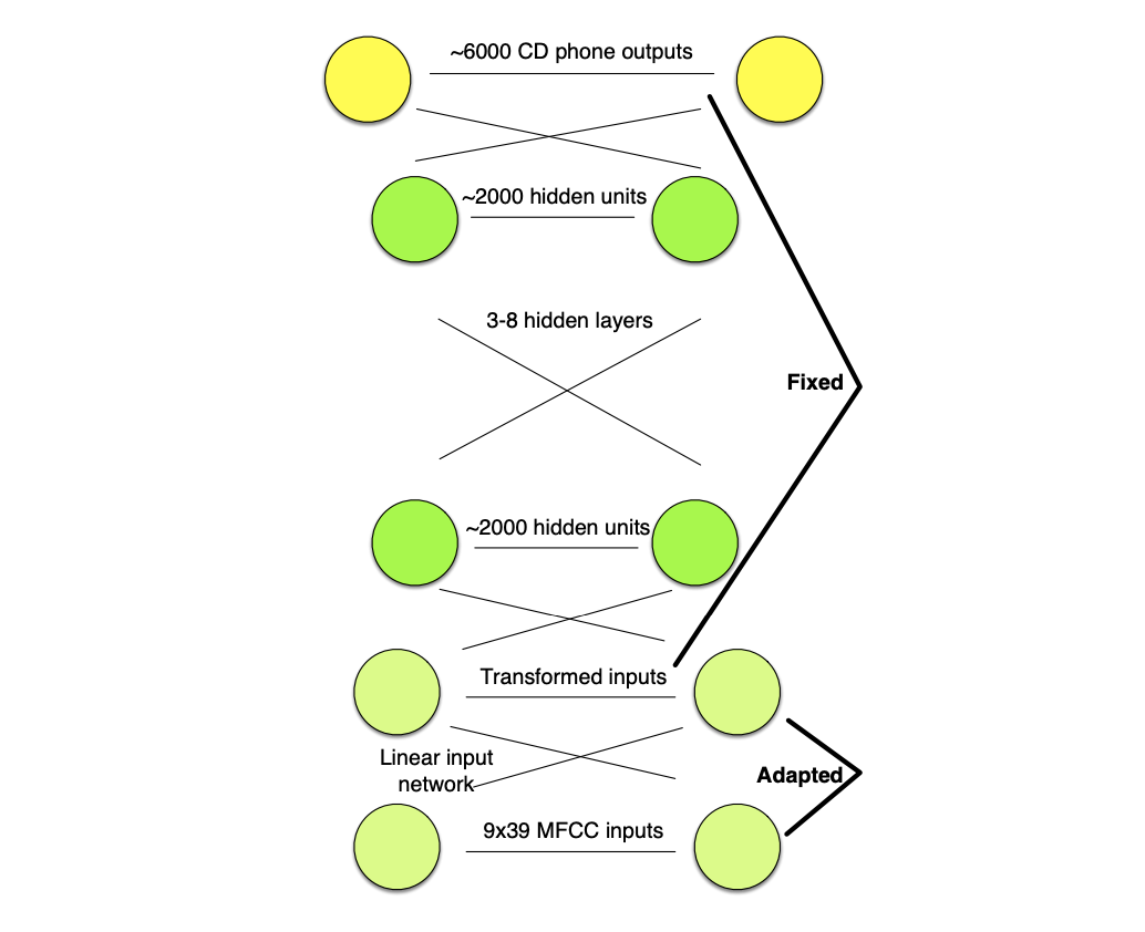
In training, the LIN is fixed and in testing, the main speaker-independent network is fixed.
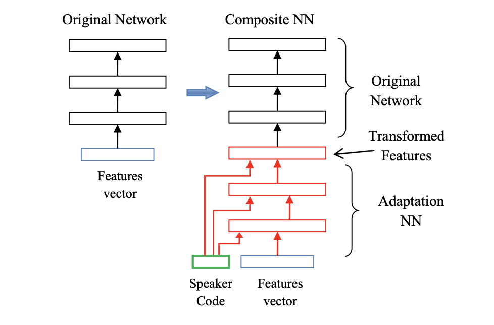
Speaker codes with i-vectors
We can also learn a short speaker code vector for talker, and combine that with the input feature vector, to compute transformed features. This allows an adaptation on speaker specific means.
i-vectors are used as speaker codes. i-vectors are fixed-dimensional representations \(\lambda_s\) for a speaker \(s\). They model the difference between the means trained on all data \(\mu_0\) and the speaker specific means \(\mu_s\):
\[ \mu_s = \mu_0 + M \lambda_S\]i-vectors are derived from a factor analysis, and widely used in speaker identification.
Learning Hidden Unit Contributions (LHUC)
In LHUC, we add a learnable speaker dependent amplitude to each hidden unit, which allows us to learn amplitudes from data, per speaker, and it “embeds” in a sense the adaptation part.
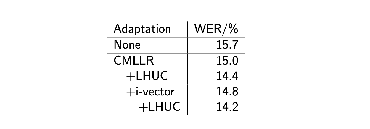
Below are the results, in terms of WER, of various adaptation methods, and their combinations.
Conclusion
If you want to improve this article or have a question, feel free to leave a comment below :)
References: