
So far, we have covered HMM-GMM acoustic modeling and some practical issues related to context and less frequent phonemes.
Introduction to Neural Network acoustic modeling
There is an alternative way to build an acoustic model, and it consists in using neural networks to:
- take an input acoustic frame
- and output a score for each phone
Let’s consider a single-layer neural network, that takes as an input an acoustic frame \(X_t\) and outputs phonetic scores \(f(t)\) (one score for each phone).
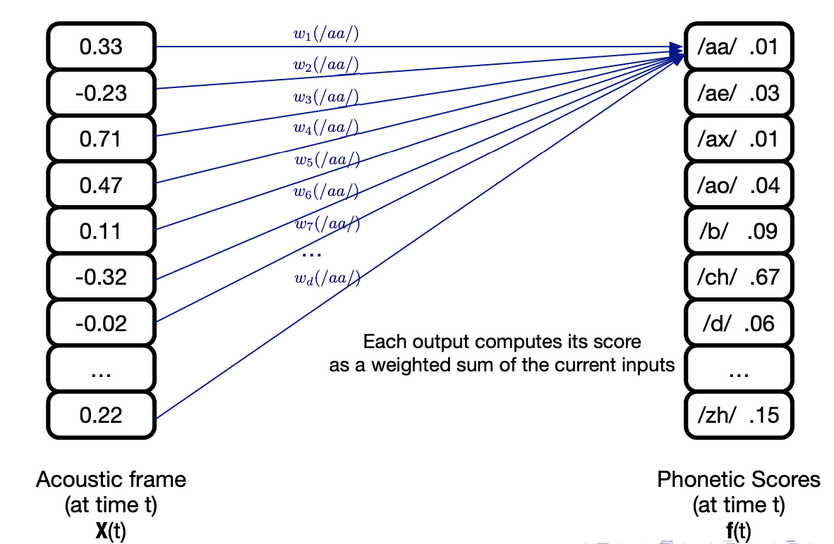
It can be expressed as:
\[f = Wx + b\]Where \(W\) is the weight matrix made of weights \(w_{ij}\) that reflect the weifht between input \(i\) and output \(j\), and \(b\) is the bias term.
How do we learn the parameters \(W\) and \(b\)? We target the minimization of the error function \(E\), the Mean Square Error (MSE) between the output and the target:
\[E = 0.5 \times \frac{1}{T} \sum_{t=1}^T {\mid \mid f(x_t) - r(t) \mid \mid}^2\]Where \(r(t)\) are the target outputs.
The error minimization is typically done using gradient descent, and we must compute the terms:
\(\frac{d E}{d W}\) and \(\frac{d E}{d b}\)
Reminder: Stochastic gradient descent (SGD)
In SGD, we:
- intialize weights and biases with small random numbers
- randomise the order of training data example
- then for each epoch:
- take a minibact
- compute network outputs
- backpropagate and update the weights
The network that predicts phonetic scores is a classifier, so we need to take a softmax to force output values to act as probabilities:
\[y_j = \frac{exp(f(x_j))}{\sum_{k=1}^K exp(f(x_k))}\]Where \(f(x_j) = \sum_{d=1}^D w_{jd} x_d + b_j\)
However, the MSE is not the wisest choice when working with probabilities. We can directly maximize the log probability of observing the correct label using the Cross-Entropy (CE) error function:
\[E_t = - \sum{j=1}^J r_j^t \ln y_j^t\]Using CE, the gradients of the outputs weights simplify to:
\[\frac{dE^t}{dW_{jd}} = (y_j^t - r_j^t) x_d\]There are several extensions possible to this very very simple model:
- use more context by taking multiple frames into account
- add more hidden layers to obtains DNNs
- use activation functions such as ReLU
This looks interesting, and overall simpler than the HMM-GMM. But there is a major limitation, since we cannot do speech recognition with this approach. There are several phone recognition tasks:
- frame classification: classify each frame of data
- phone classification: classify each segment of data (what Neural Networks can do)
- phone recongition: segment the data and label the segment
Using only DNN, we lack the notion of data segmentation that HMMs are good at doing. But can’t we mix HMMs and DNNs ?
HMM-DNN acoustic modeling
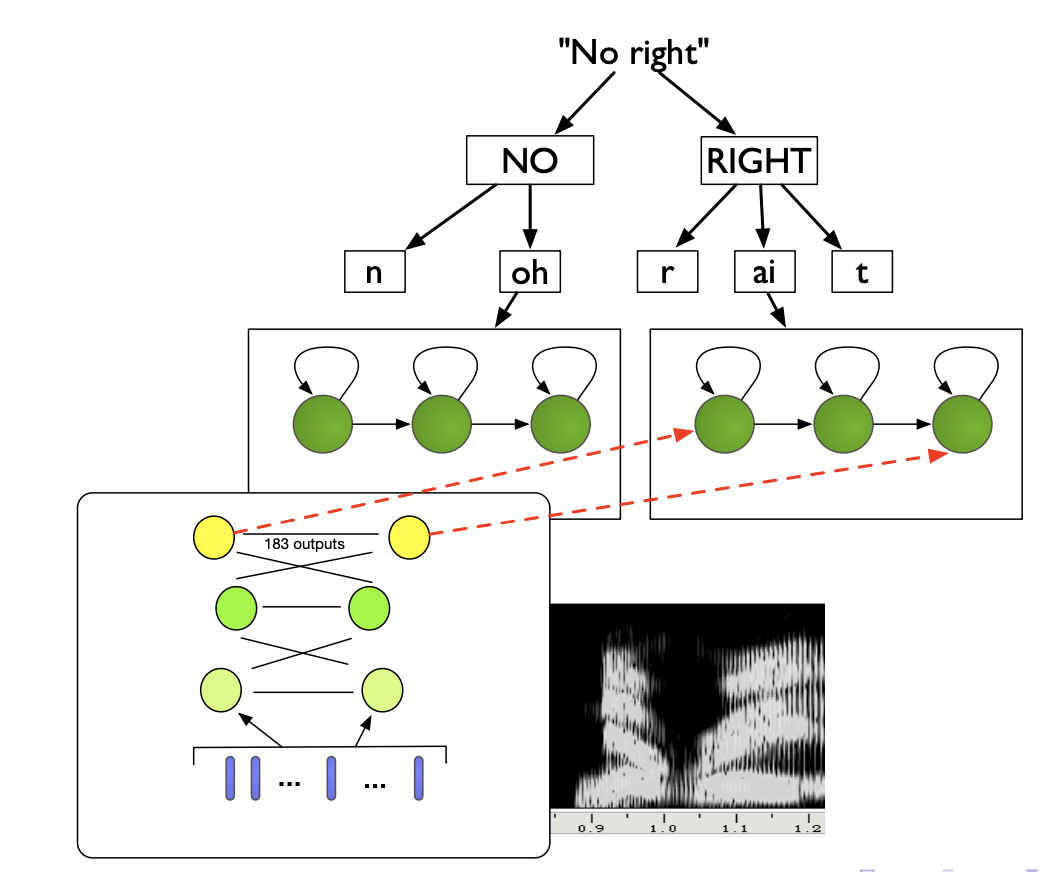
In an HMM-GMM, replacing the GMM by a DNN to estimate output pdfs build a so-called HMM-DNN architecture. In a HMM-DNN, we consider one-state per phone, and train a NN as a phone-state classifier.
It can be shown that the outputs corresponding to class \(j\) given an input \(x_t\) are an estimate of the posterior probability \(P(q_t = j \mid x_t)\), \(q_t\) being a state, because we have softmax outputs and use a CE loss function.
And using Bayes Rule, we can relate the posterior \(P(q_t = j \mid x_t)\) to the likelihood \(P(x_t \mid q_t = j)\):
\[P(q_t \mid x_t) = \frac{P(x_t \mid q_t = j) P(q_t = j)}{P(X_t)}\]If we want HMM-DNNs to output probabilities, we should scale the likelihoods:
\[\frac{P(q_t = j \mid x_t)}{P(q_t = j)} = \frac{P(x_t \mid q_t = j)}{P(x_t)}\]This means we can obtain scaled likelihoods by dividing each network output by the prior, i.e. the relative frequency of class \(j\) in training data.
There are several approaches to continuous speech recognition with HMM-DNN:
- 1 state per phone (each NN can output typically 60 classes if 60 phone classes)
- 3 state context-independent (CI) models, where each phone has 3 states, modeled by 3 NNs
- State-clustered context-dependent (CD) models, 1 NN output per tied state
The architecture of a HMM-DNN is presented below:
NN are more flexible, learn richer representations and handle correlated features. In terms of speech features, experiments indicate that mel-scaled filter bank features (FBANK) work better than MFCCs, and results in better clustering when applying t-SNE on the hidden layers. Indeed, in FBANK the useful information is distributed over all the features, whereas in MFCC it is concentrated in the first few.
Modelling phonetic context with DNNs
Modling the phonetic context with DNNs was considered hard until 2011, but a simple solution emerged: use the state-tying process from a GMM system, and train a HMM-DNN on it.
More precisely, the context-dependent hybrid HMM/DNN approach is:
- Train a GMM/GMM system on your data
- Use a phonetic decision tree to determine the HMM tied states for infrequent states
- Perform Viterbi alignment using the trained HMM/GMM and the training data
- Train a neural network to map the input speech features to a label representing a context-dependent tied HMM-state, instead of contenxt-independent phones
- this increases the number of possible labels, and each frame is labelled with Viterbi aligned tied states
- we then train the NN using gradient descent
Concretely, we model the acoustic context by including neighbour frames in the input layer.
We use richer Neural Network models for acoustic context:
- Recurrent Neural Networks (RNNs)
- Time-delay Neural Networks (TDNNs)
Time-delay Neural Networks
In TDNNs, higher hidden layers take input from a larger acoustic context, and lower hidden layers from narrower contexts. TDNNs can be seen as a 1D convolutional network.
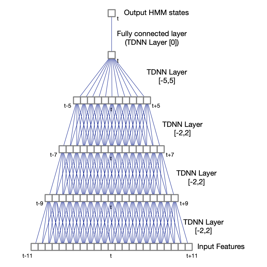
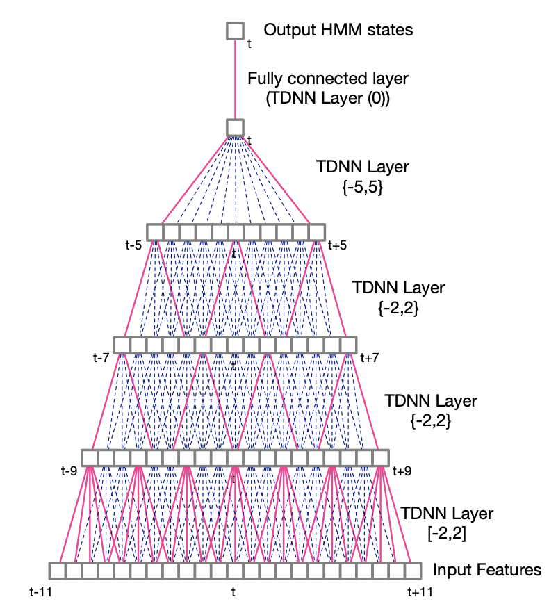
A TDNN with a context (-2, 2) has 5 times more weights than a regular DNN. For this reason, sub-sampled TDNNs are explored. Due to the large overlaps between input contexts at adjacent time steps, which are likely to be correlated, we take a sub-sample window of hidden unit activations. It reduces computation time and model weights.
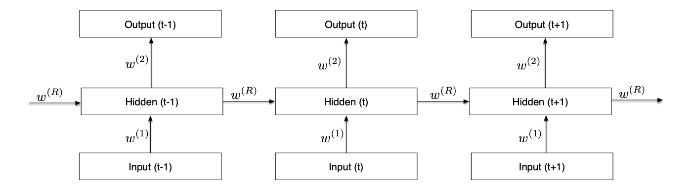
Recurrent Neural Networks
In its unfolded representation, the RNN for a sequence of T inputs is a T-layer network with shared weights. It can keep information through time.
LSTMs avoid the vanishing gradient problem of RNNs. Bidirectional RNNs consider both the right and the left context, in a forward layer and a backward layer. Deep RNNs have several hidden layers, and deep bidirectional LSTM combine the advantages of all these methods:
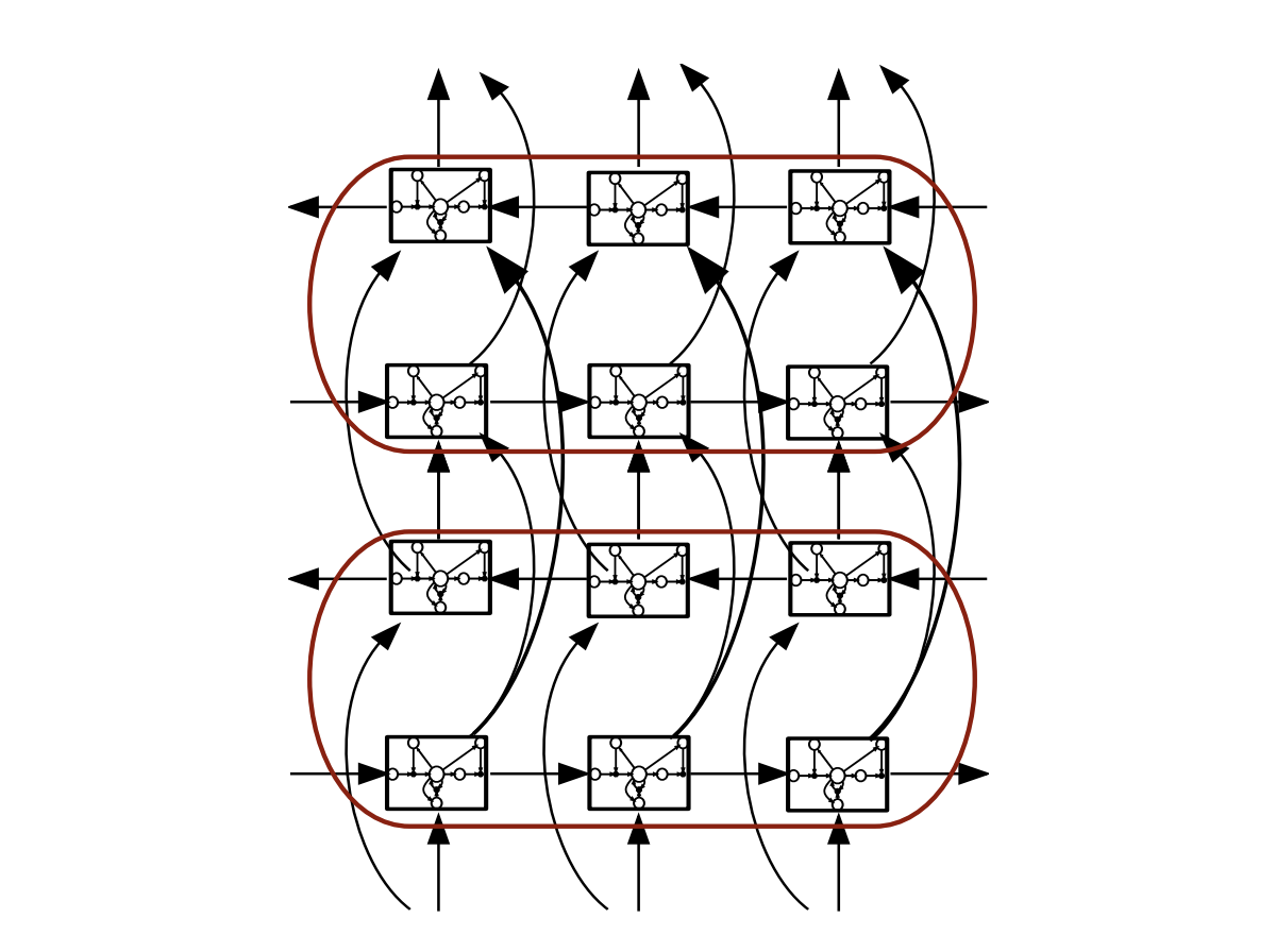
Here is an example of a Bidirectional LSTM Acoustic Model training on the Switchboard dataset:
- LSTM has 4-6 bidirectional layers with 1024 cells/layer (512 each direction)
- 256 unit linear bottleneck layer
- 32k context-dependent state outputs
- Input features:
- 40-dimension linearly transformed MFCCs (plus ivector)
- 64-dimension log mel filter bank features (plus first and second derivatives)
- concatenation of MFCC and FBANK features
- Training: 14 passes frame-level cross-entropy training, 1 pass sequence training (2 weeks on a K80 GPU)
LSTMs + feature fusion currently reach close to state-of-the-art.
Conclusion
If you want to improve this article or have a question, feel free to leave a comment below :)
References: