
Let’s now dive into acoustic modeling, with the historical approach: Hidden Markov Models and Gaussian Mixture Models (HMM-GMM).
Introduction to HMM-GMM acoustic modeling
Rather than covering into the maths of HMMs and GMMs in this article, I would like to invite you to read these slides that I have made on the topic of Expectation Maximization for HMMs-GMMs, it starts from very basic concepts and covers up to the end. Before going through the slides, let us just remind us what we try to do here.
We want to cover the acoustic modeling, meaning that the HMM-GMM will model \(P(X \mid W)\) in the diagram below.
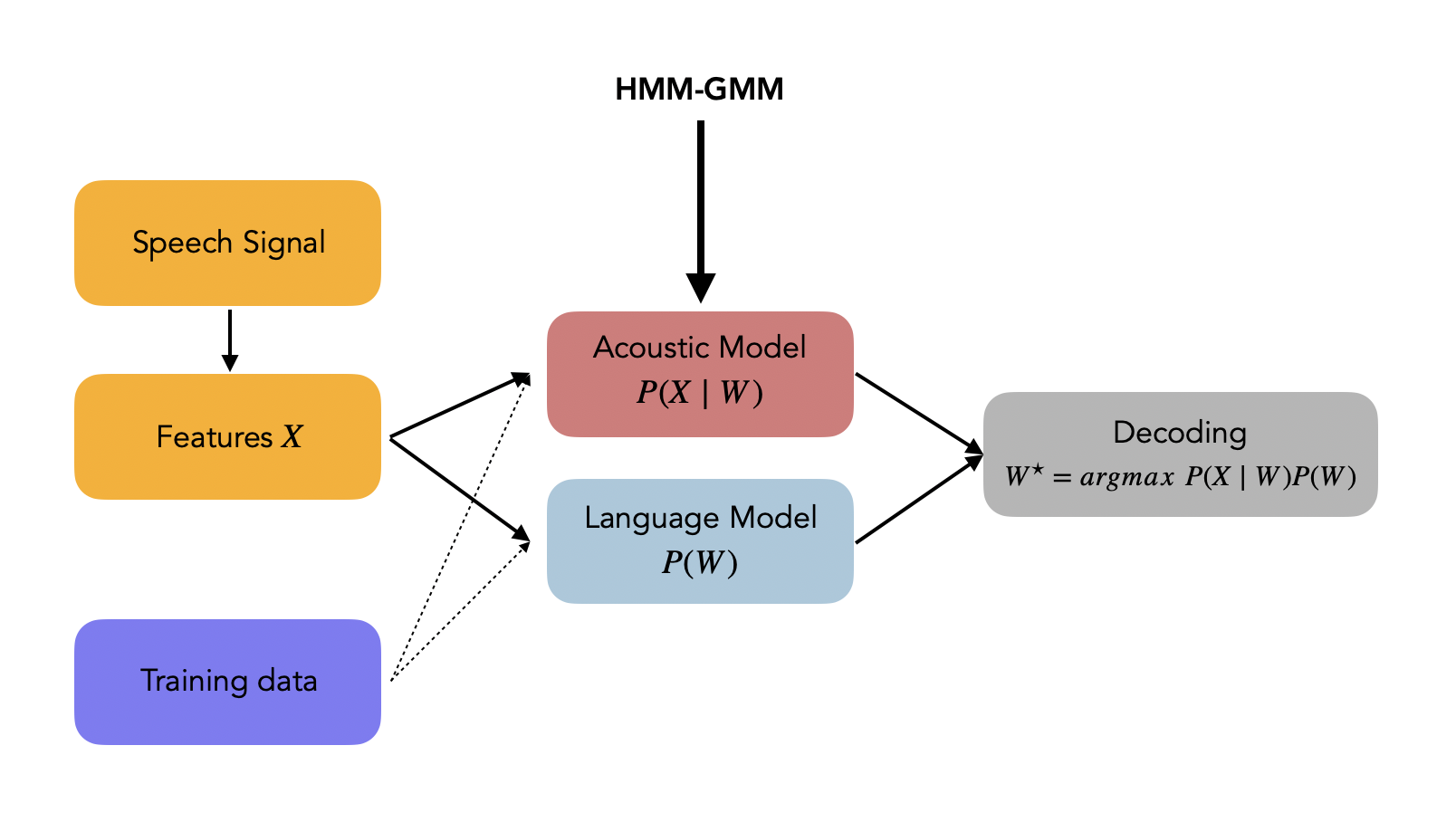
In the ASR course of the University of Edimburgh, this diagram illustrates where this HMM-GMM architecture takes place:
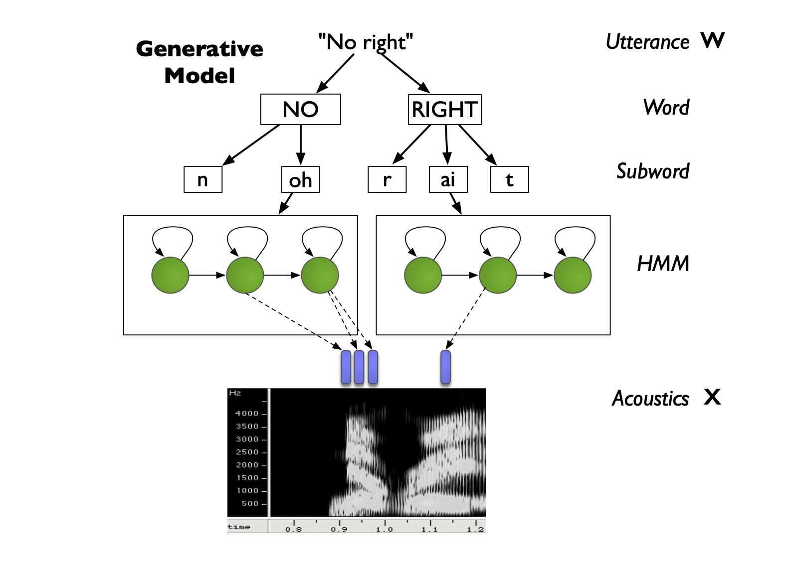
From the utterance \(W\), we can break it down into words, then into subwords (or phonemes or phones), and we represent each subword as a HMM. Therefore, for each subword, we have a HMM with several hidden states, which generates features based on a GMM at each state, and these features will represent the acoustic features \(X\).
Alright, let’s jump to the slides:
If you follow the ASR course of the University of Edimburgh, the slides above will correspond to:
Context-dependent phone models
Overview
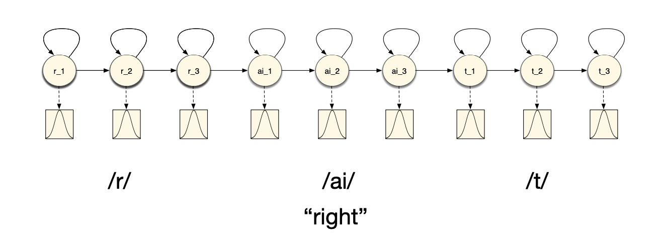
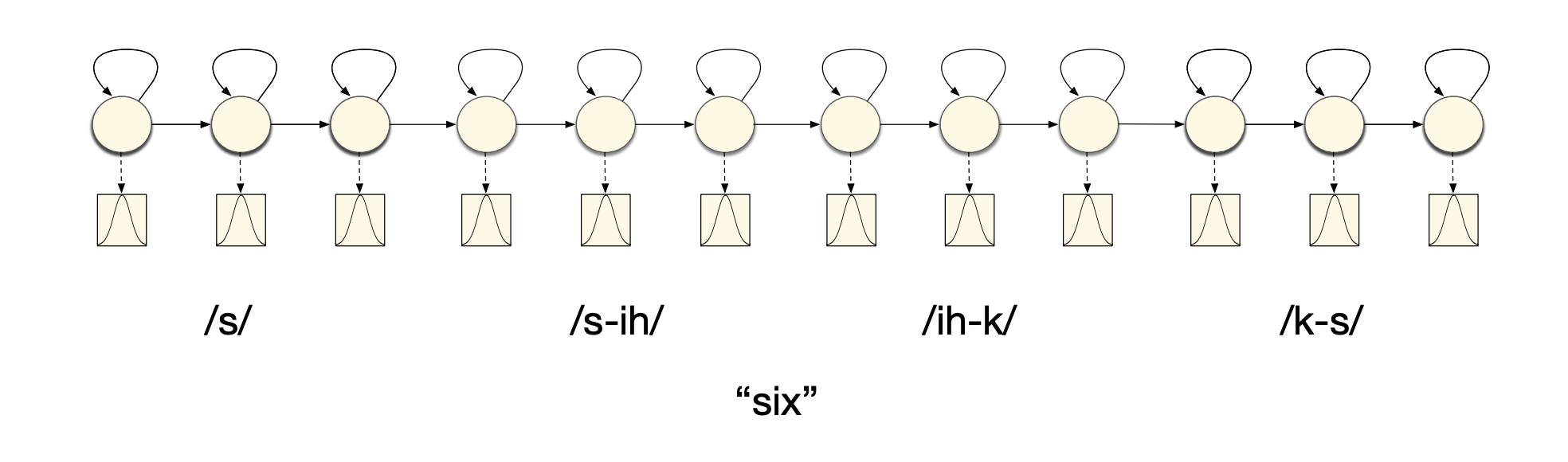
As seen in the slides, there are several ways to model words with HMM models. We can either consider that a single phone is represented by several hidden states of a HMM:
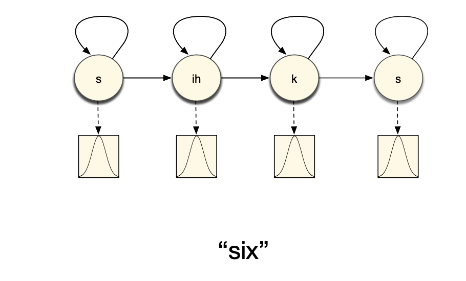
Or that each phone is modeled by a single state of a HMM:
The acoustic phonetic context of a speech unit describes how articulation (acoustic realization) changes depending on the surrounding units. For example, “/n/” is not pronounced the same in “ten” (alveolar) and “tenth” (dental).
And this violates the Markov assumption of the acoustic realization being independent of the previous states. But how can we model context?
- using pronounciations, hence leading to a pronounciation model
- using subwords units with context:
- use longer units that incorporate context, e.g. biphones or triphones, demisyllables or syllables
- use multiples models for each
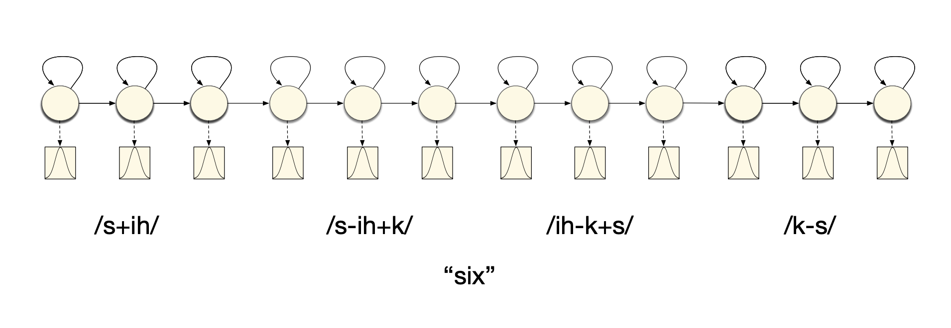
For example, left biphones modeling would look like this:
And triphones can be represented this way:
Context dependent models are:
- more specific
- can define multiple context-dependent models to increase the state-space
- handles incorrectness of Markov assumption
- each model is now responsible for a smaller region of the acoustic-phonetic space
Triphones models
There are 2 main types of triphones:
- word-internal triphones: we only take triphones within a word
- cross-word triphones: triphones can model the links between words too
If we have a system with 40 phones, then the total number of triphones that can occur is: \(40^4 = 64000\). In a cross-word system, typicall 50’000 of them can occur.
The number of gaussians of 50’000 3-states HMMs with 10 components per gaussian is 1.5 million. If features are 39-dimensional (12 MFCCs + energy, delta and accelaration), then each Gaussian has 790 parameters, leading to 118 million parameters! We need huge amount of training data, which ensures that all combinations are covered. Otherwise, we can explore alternatives.
Modeling infrequent triphones
There are several ways to handle infrequent triphones rather than expecting large amount of training data:
- smoothing
- parameter sharing
Smoothing
In smoothing back-off, the idea is to use less specific models when there’s not enough data to train a specific model. If a triphone is not observed enough, we can use a biphones, or even a monophones.
On the other hand, in smoothing interpolation, the idea is to combine less specific models with more specific ones, e.g. :
\[\hat{\lambda}^{tri} = \alpha_3 \lambda^{tri} + \alpha_2 \lambda^{bi} + \alpha_1 \lambda^{mono}\]Interpolation allows more triphone models to be estimated, and adds robustness by sharing data from other contexts.
Parameter sharing
One of the most common ones is parameter sharing, where different contexts share models. This can be done in 2 ways:
- bottom-up: start with all possible contexts, and merge them progressively
- top-down: start with a single global context, and split progressively
Sharing can take place at different levels:
-
Sharing Gaussians, where all distributions share the same set of Gaussians but have different mixture weights, called tied mixtures.
-
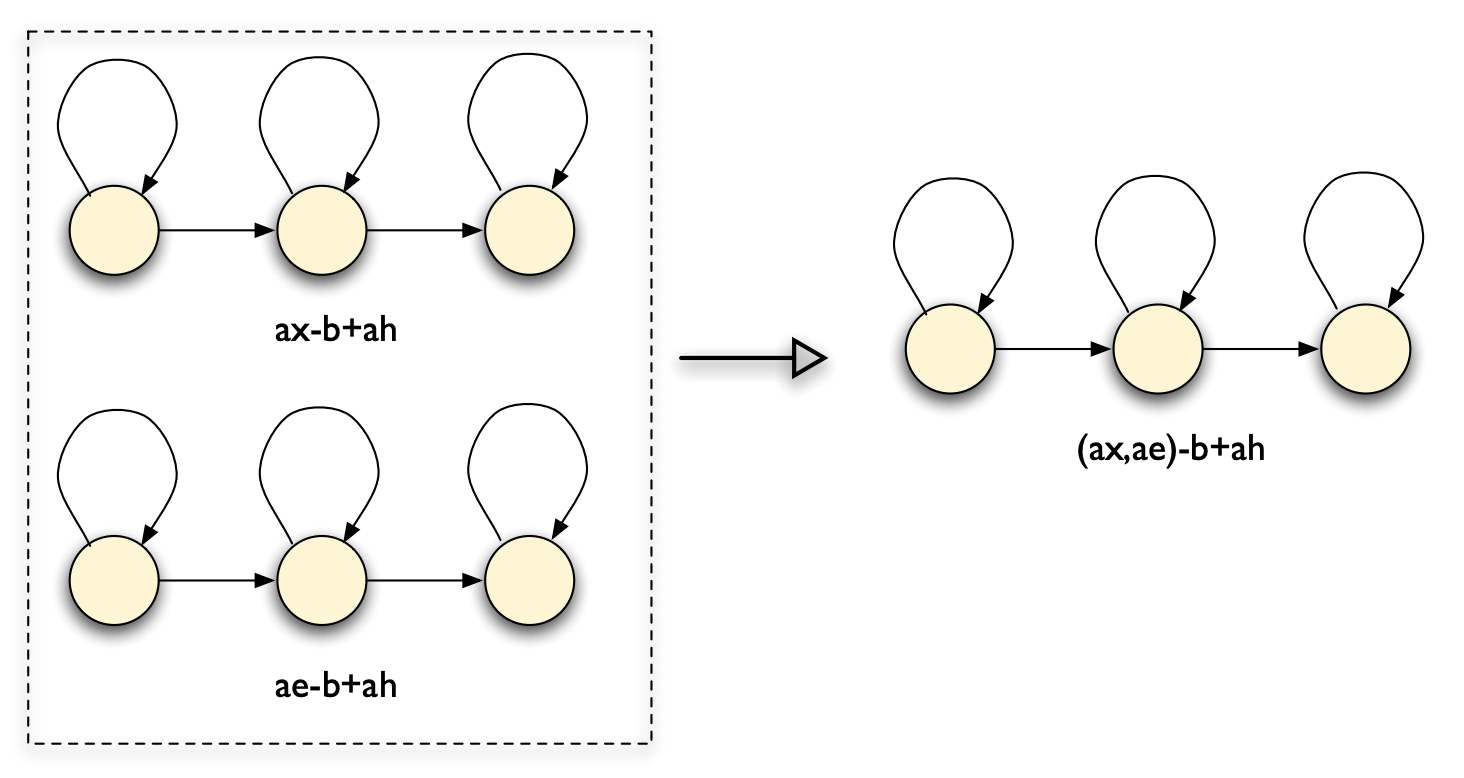
Sharing models: merge context-dependent models that are most similar, called generalised triphones
Generalised triphones are illustrated below. These type of models are more accurate, since trained on more data.
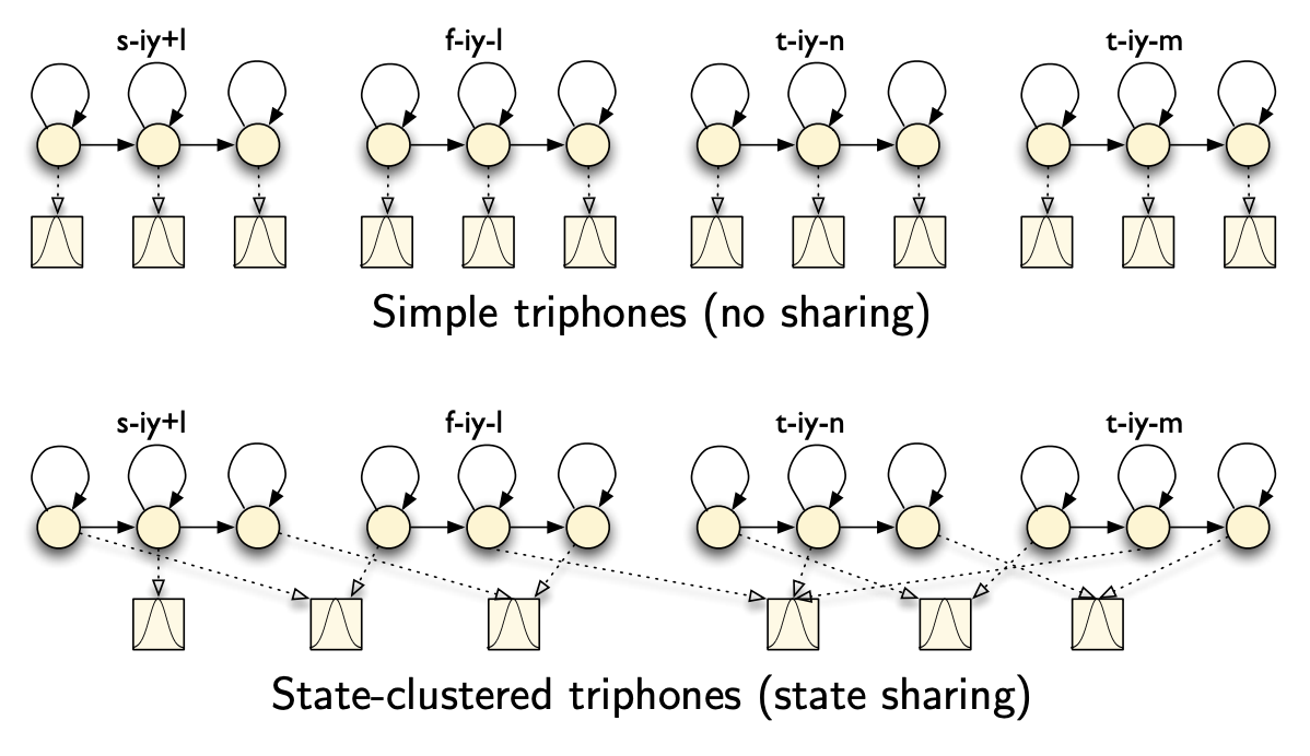
- Sharing states: different models that the same states, called state clustering. This is what is implemented in Kaldi.
But how do we decide which states to cluster together?
- Bottom-up: create raw triphone models and cluster states. But unable to solve unseen triphone problems.
- Top-down clustering: start with a parent context independent model and split successively to create context dependent models. The aim is to increase the likelihood by splitting : \(Gain = L(S_1) + L(S_2) - L(S)\)
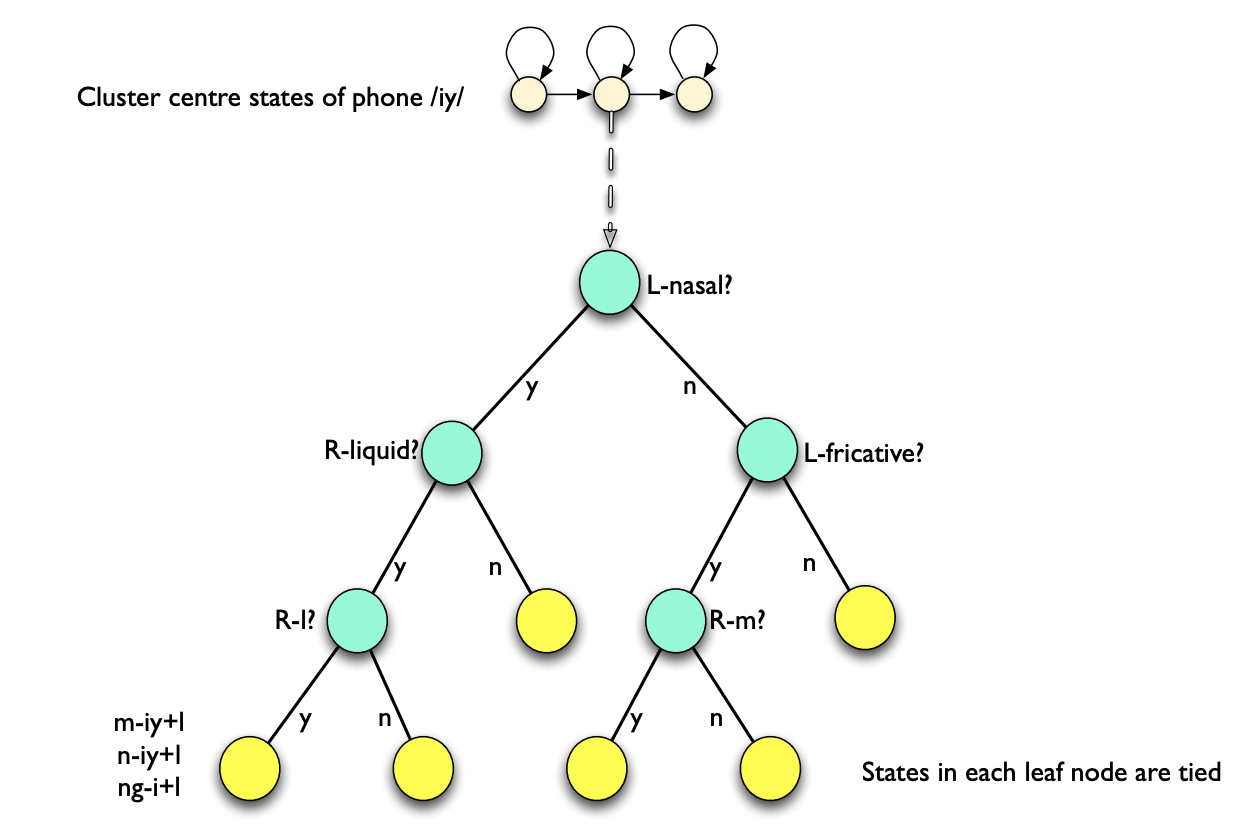
But then the question becomes: How to find the best splits? This is done using phonetic decision trees. At the root od the tree, all states are shared. Then, using questions, we split the pool of states, and create leves of the tree. The questions might for example be:
- is left context a nasal?
- is right context a central stop?
We choose the question that maximizes the likelihood of the data given the state clusters, and stop if the likelihood does not increase more than a threshold, or the amount of data in a split is not sufficient enough (like a normal decision tree).
In Kaldi, it generates questions automatically using a top down binary clustering. Another question remains: How do you compute the log-likelihood of a state cluster?
If you consider a cluster \(S\) made of \(K\) states forming the cluster, all of them sharing a common mean \(\mu_S\) and covariance \(\Sigma_S\), and training data \(X\) generated with probability \(\gamma_S(X)\) by state \(s\), then the likelihood of the state cluster is given by:
\[L(S) = \sum_{s \in S} \sum_{x \in X} log P(x \mid \mu_S, \Sigma_S) \gamma_S(x)\]And if the output pdfs are Gaussian, it can be shown that:
\[L(S) = - \frac{1}{2} (log ( (2 \pi)^d \mid \Sigma_S \mid ) + d) \sum_{s \in S} \sum_{x \in X} \gamma_S(x)\]And hence, \(L(S)\) only depends on the pooled state variance \(\Sigma_S\) and the state occupation probability (known from the forward-backward iterations).
In summary, the process applied in Kaldi is:
- share parmeters through state clustering
- cluster states using phonetic decision tree (with the gaussian assumption)
- split gaussians and re-train to obtain a GMM state clustered system
Conclusion
If you want to improve this article or have a question, feel free to leave a comment below :)
References: