This article provides a summary of the course “Automatic speech recognition” by Gwénolé Lecorvé from the Research in Computer Science (SIF) master, to which I added notes of the Statistical Sequence Processing course of EPFL, and from some tutorials/personal notes. All references are presented at the end.

Introduction to ASR

What is ASR?

Automatic Speech Recognition (ASR), or Speech-to-text (STT) is a field of study that aims to transform raw audio into a sequence of corresponding words.

Some of the speech-related tasks involve:

speaker diarization: which speaker spoke when?
speaker recognition: who spoke?
spoken language understanding: what’s the meaning?
sentiment analysis: how does the speaker feel?

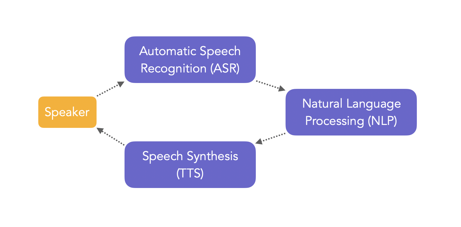
The classical pipeline in an ASR-powered application involves the Speech-to-text, Natural Language Processing and Text-to-speech.

ASR is not easy since there are lots of variabilities:

acoustics:
- variability between speakers (inter-speaker)
- variability for the same speaker (intra-speaker)
- noise, reverberation in the room, environment…
phonetics:
- articulation
- elisions (grouping some words, not pronouncing them)
- words with similar pronounciation
linguistics:
- size of vocabulary
- word variations
- …

From a Machine Learning perspective, ASR is also really hard:

very high dimensional output space, and a complex sequence to sequence problem
few annotated training data
data is noisy

How is speech produced?

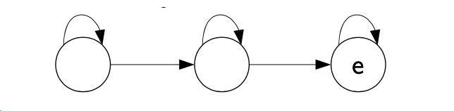
Let us first focus on how speech is produced. An excitation \(e\) is produced through lungs. It takes the form of an initial waveform, describes as an airflow over time.

Then, vibrations are produced by vocal cords, filters \(f\) are applied through pharynx, tongue…

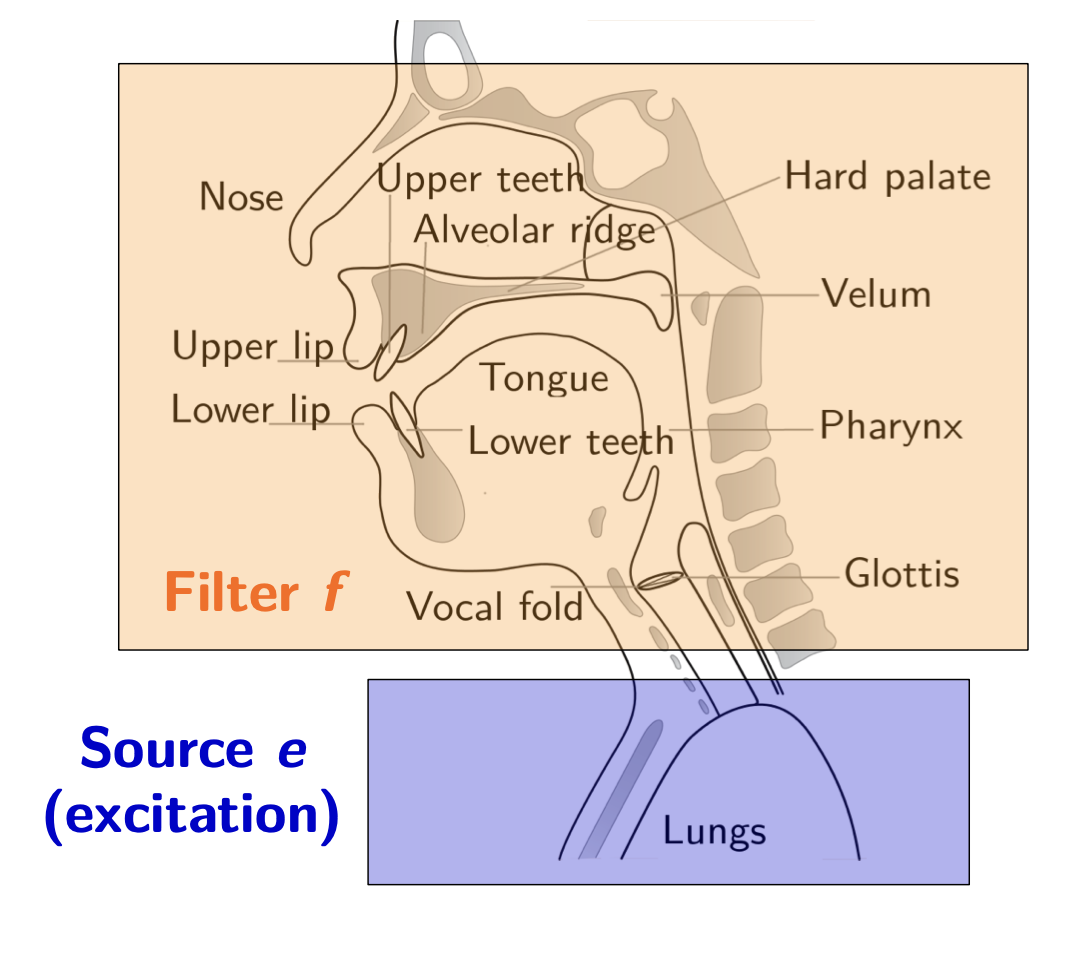
The output signal produced can be written as \(s = f * e\), a convolution between the excitation and the filters. Hence, assuming \(f\) is linear and time-independent:

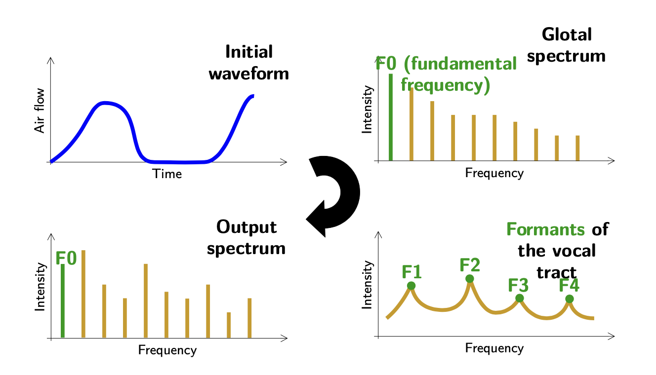
\[s(t) = \int_{-\infty}^{+\infty} e(t) f(t-\tau)d \tau\]

From the initial waveform, we generate the glotal spectrum, right out of the vocal cords. A bit higher the vocal tract, at the level of the pharynx, pitches are formed and produce the formants of the vocal tract. Finally, the output spectrum gives us the intensity over the range of frequencies produced.

Breaking down words

In automatic speech recognition, you do not train an Artificial Neural Network to make predictions on a set of 50’000 classes, each of them representing a word.

In fact, you take an input sequence, and produce an output sequence. And each word is represented as a phoneme, a set of elementary sounds in a language based on the International Phonetic Alphabet (IPA). To learn more about linguistics and phonetic, feel free to check this course from Harvard. There are around 40 to 50 different phonemes in English.

Phones are speech sounds defined by the acoustics, potentially unlimited in number,

For example, the word “French” is written under IPA as : / f ɹ ɛ n t ʃ /. The phoneme describes the voiceness / unvoiceness as well as the position of articulators.

Phonemes are language-dependent, since the sounds produced in languages are not the same. We define a minimal pair as two words that differ by only one phoneme. For example, “kill” and “kiss”.

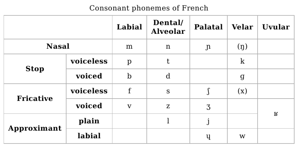
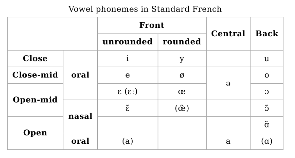
For the sake of completeness, here are the consonant and vowel phonemes in standard french:

There are several ways to see a word:

as a sequence of phonemes
as a sequence of graphemes (mostly a written symbol representing phonemes)
as a sequence of morphemes (meaningful morphological unit of a language that cannot be further divided) (e.g “re” + “cogni” + “tion”)
as a part-of-speech (POS) in morpho-syntax: grammatical class, e.g noun, verb, … and flexional information, e.g singular, plural, gender…
as a syntax describing the function of the word (subject, object…)
as a meaning

Therefore, labeling speech can be done at several levels:

word
phones
…

And the labels may be time-algined if we know when they occur in speech.

The vocabulary is defined as the set of words in a specific task, a language or several languages based on the ASR system we want to build. If we have a large vocabulary, we talk about Large vocabulary continuous speech recognition (LVCSR). If some words we encounter in production have never been seen in training, we talk about Out Of Vocabulary words (OOV).

We distinguish 2 types of speech recognition tasks:

isolated word recognition
continuous speech recognition, which we will focus on

Evaluation metrics

We usually evaluate the performance of an ASR system using Word Error Rate (WER). We take as a reference a manual transcript. We then compute the number of mistakes made by the ASR system. Mistakes might include:

Substitutions, \(N_{SUB}\), a word gets replaced
Insertions, \(N_{INS}\), a word which was not pronounced in added
Deletions, \(N_{DEL}\), a word is omitted from the transcript

The WER is computed as:

\[WER = \frac{N_{SUB} + N_{INS} + N_{DEL}}{\mid N_{words-transcript} \mid}\]

The perfect WER should be as close to 0 as possible. The number of substitutions, insertions and deletions is computed using the Wagner-Fischer dynamic programming algorithm for word alignment.

Statistical historical approach to ASR

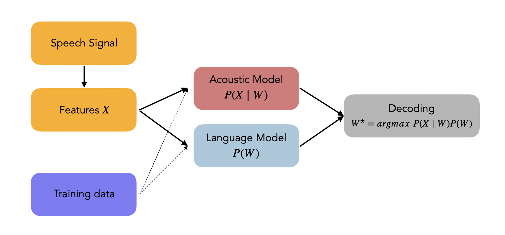
Let us denote the optimal word sequence \(W^{\star}\) from the vocabulary. Let the input sequence of acoustic features be \(X\). Stastically, our aim is to identify the optimal sequence such that:

\[W^{\star} = argmax_W P(W \mid X)\]

This is known as the “Fundamental Equation of Statistical Speech Processing”. Using Bayes Rule, we can rewrite is as :

\[W^{\star} = argmax_W \frac{P(X \mid W) P(W)}{P(X)}\]

Finally, we suppose independence and remove the term \(P(X)\). Hence, we can re-formulate our problem as:

\[W^{\star} = argmax_W P(X \mid W) P(W)\]

Where:

\(argmax_W\) is the search space, a function of the vocabulary
\(P(X \mid W)\) is called the acoustic model
\(P(W)\) is called the language model

The steps are presented in the following diagram:

Feature extraction \(X\)

From the speech analysis, we should extract features \(X\) which are:

robust across speakers
robust against noise and channel effects
low dimension, at equal accuracy
non-redondant among features

Features we typically extract include:

Mel-Frequency Cepstral Coefficients (MFCC), as desbribed here
Perceptual Linear Prediction (PLP)
…

We should then normalize the features extracted to avoid mismatches across samples with mean and variance normalization.

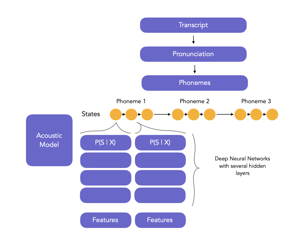
Acoustic model

1. HMM-GMM acoustic Model

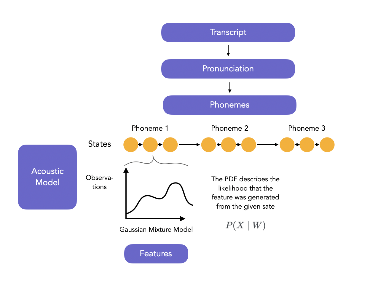
The acoustic model is a complex model, usually based on Hidden Markov Models and Artificial Neural Networks, modeling the relationship between the audio signal and the phonetic units in the language.

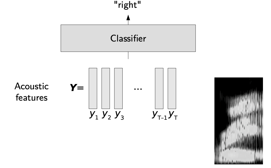
In isolated word/pattern recognition, the acoustic features (here \(Y\)) are used as an input to a classifier whose rose is to output the correct word. However, we take input sequence and should output sequences too when it comes to continuous speech recognition.

The acoustic model goes further than a simple classifier. It outputs a sequence of phonemes.

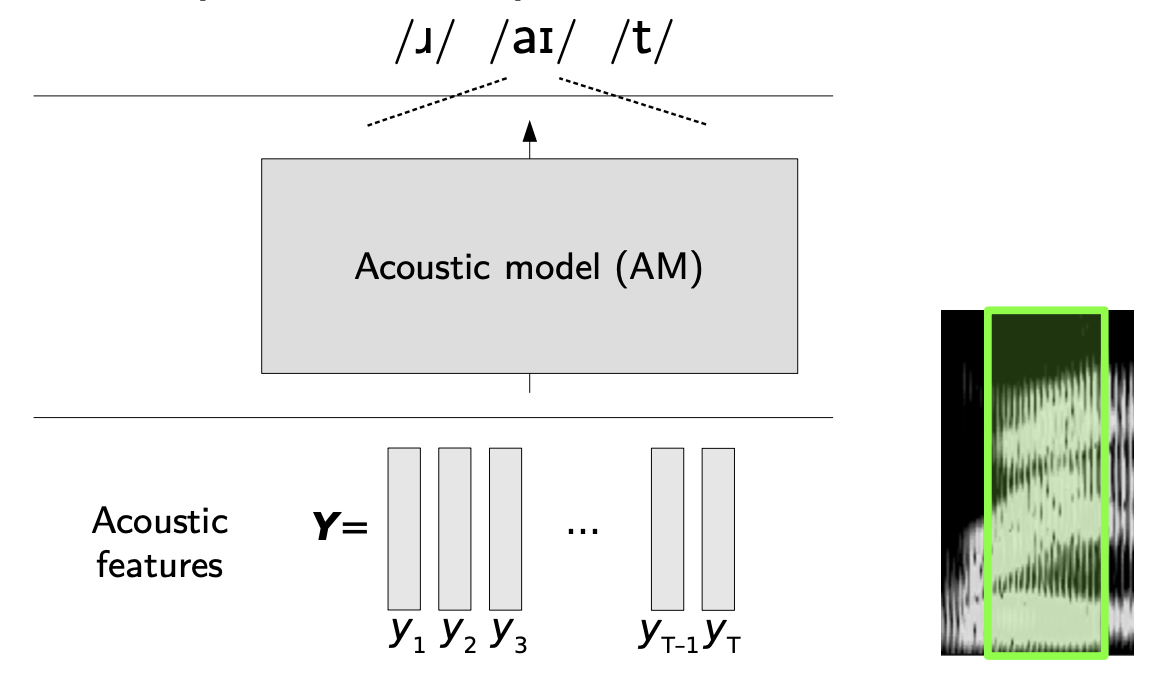
Hidden Markov Models are natural candidates for Acoustic Models since they are great at modeling sequences. If you want to read more on HMMs and HMM-GMM training, you can read this article. The HMM has underlying states \(s_i\), and at each state, observations \(o_i\) are generated.

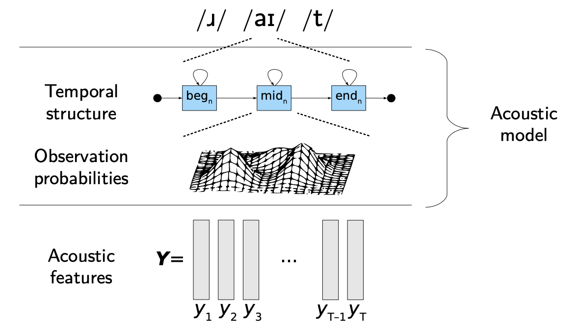
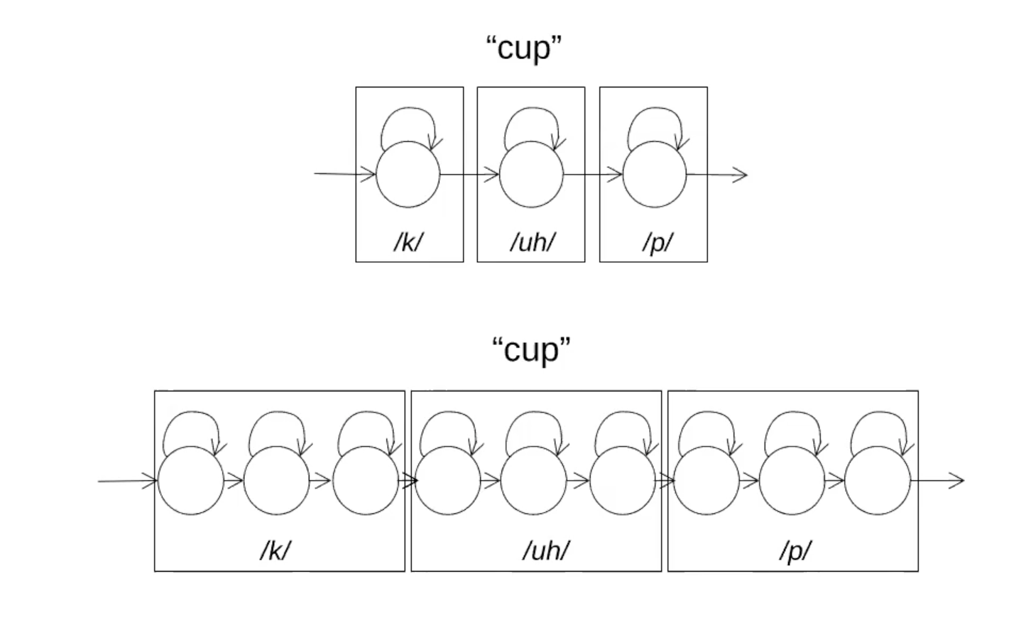
In HMMs, 1 phoneme is typically represented by a 3 or 5 state linear HMM (generally the beginning, middle and end of the phoneme).

The topology of HMMs is flexible by nature, and we can choose to have each phoneme being represented by a single state, or 3 states for example:

The HMM supposes observation independence, in the sense that:

\[P(o_t = x \mid s_t = q_i, s_{t-1} = q_j, ...) = P(o_t = x \mid s_t = q_i)\]

The HMM can also output context-dependent phonemes, called triphones. Triphones are simply a group of 3 phonemes, the left one being the left context, and the right one, the right context.

The HMM is trained using Baum-Welsch algorithm. The HMMs learns to give the probability of each end of phoneme at time t. We usually suppose the observations are generated by a mixture of Gaussians (Gaussian Mixture Models, GMMs) at each state, i.e:

\[P(o_t = y \mid s_t = q_i) = P(X \mid W) = \sum_{m=1} \mathcal{N}(y, \mu_{jm}, \Sigma_{jm})\]

The training of the HMM-GMM is solved by Expectation Maximization (EM). In the EM training, the outputs of the GMM \(P(X \mid W)\) are used as inputs for the GMM training iteratively, and the Viterbi or Baum Welsch algorithm trains the HMM (i.e. identifies the transition matrices) to produce the best state sequence.

The full pipeline is presented below:

2. HMM-DNN acoustic model

Latest models focus on hybrid HMM-DNN architectures and approach the acoustic model in another way. In such approach, we do not care about the acoustic model \(P(X \mid W)\), but we directly tackle \(P(W \mid X)\) as the probability of observing state sequences given \(X\).

Hence, back to the first acoustic modeling equation, we target:

\[W^{\star} = argmax_W P(W \mid X)\]

The aim of the DNN is to model the posterior probabilities over HMM states.

Some considerations on the HMM-DNN framework:

we usually take a large number of hidden layers
the inputs features typically are extracted from large windows (up to 1-2 seconds) to have a large context
early stopping can be used

You might have noticed that the training of the DNN produces posterior, whereas the Viterbi Backward-Forward algorithm requires \(P(X \mid W)\) to identify the optimal sequence when training the HMM. Therefore, we use Bayes Rule:

\[P(X \mid W) = \frac{P(W \mid X) P(X)}{P(W)}\]

The probability of the acoustic feature \(P(X)\) is not known, but it just scales all the likelihoods by the same factor, and therefore does not modify the alignment.

The training of HMM-DNN architectures is based:

either on the original hybrid HMM-DNN, using EM, where:
- E-step keeps DNN and HMM parameters constant and estimates the DNN outputs to produce scaled likelihoods
- M-step re-trains the DNN parameters on the new targets from E-step
either using REMAP, with a similar architecture, except that the states priors are also given as inputs to the DNN

3. HMM-DNN vs. HMM-GMM

Here is a brief summary of the pros and cons of HMM/DNN and HMM/GMM:

HMM/DNN	HMM/GMM
Considers short term correlation	Assumes no correlation in inputs
No probability distribution function assumption	Assumes GMMs as PDFs
Discriminative training in the generated distributions	No discriminative training in the generated distributions (can be overlapping)
Discriminative acoustic model at frame level	Poor discrimination (Maximum Likelihood instead of Maximum A Posteriori)
Higher performance	Lower performance

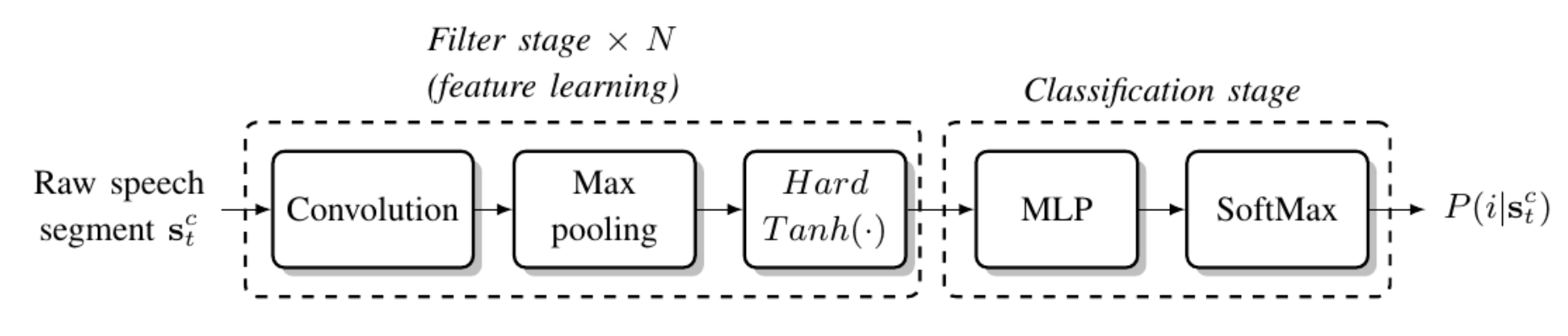
4. End-to-end models

In End-to-end models, the steps of feature extraction and phoneme prediction are combined:

This concludes the part on acoustic modeling.

Pronunciation

In small vocabulary sizes, it is quite easy to collect a lot of utterances for each word, and the HMM-GMM or HMM-DNN training is efficient. However, “statistical modeling requires a sufficient number of examples to get a good estimate of the relationship between speech input and the parts of words”. In large-vocabulary tasks, we might collect 1 or even 0 training examples. t. Thus, it is not feasible to train a model for each word, and we need to share information across words, based on the pronunciation.

\[W^{\star} = argmax_W P(W \mid X)\]

We consider words are being sequences of states \(Q\).

\[W^{\star} = argmax_W P(X \mid Q, W) P(Q, W)\] \[W^{\star} \approx argmax_W P(X \mid Q) \sum_Q P(Q \mid W) P(W)\] \[W^{\star} \approx argmax_W max_Q P(X \mid Q) P(Q \mid W) P(W)\]

Where \(P(Q \mid W)\) is the pronunciation model.

The pronunciation dictionary is written by human experts, and defined in the IPA. The pronunciation of words is typically stored in a lexical tree, a data structure that allows us to share histories between words in the lexicon.

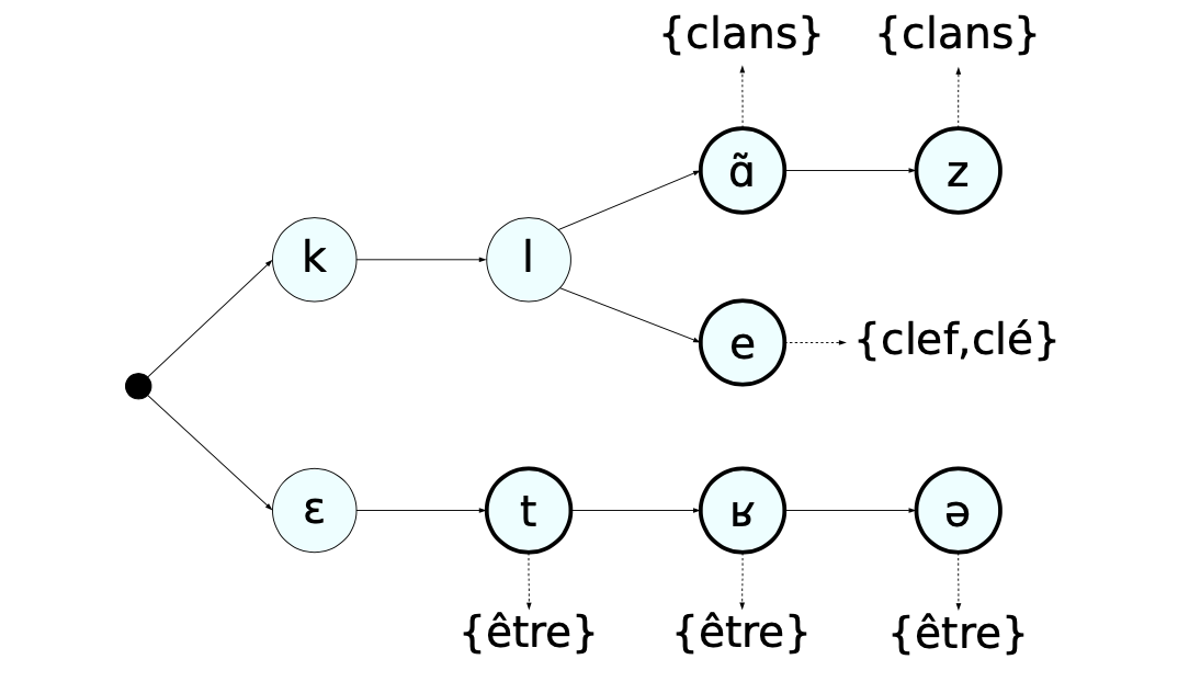
When decoding a sequence in prediction, we must identify the most likely path in the tree based on the HMM-DNN output.

In ASR, most recent approaches are:

either end to end
or at the character level

In both approaches, we do not care about the full pronunciation of the words. Grapheme-to-phoneme (G2P) models try to learn automatically the pronunciation of new words.

Language Modeling

Let’s get back to our ASR base equation:

\[W^{\star} = argmax_W P(W \mid X)\] \[W^{\star} = argmax_W P(X \mid W) P(W)\]

The language model is defined as \(P(W)\). It assigns a probability estimate to word sequences, and defines:

what the speaker may say
the vocabulary
the probability over possible sequences, by training on some texts

The contraint on \(P(W)\) is that \(\sum_W P(W) = 1\).

\[W^{\star} = argmax_W P(X \mid Q, W) P(Q, W)\]

In statistical language modeling, we aim to disambiguate sequences such as:

“recognize speech”, “wreck a nice beach”

The maximum likelihood estimation of a sequence is given by:

\[P(w_i \mid w_1, ..., w_{i-1}) = \frac{C(w_1, ..., w_i)}{\sum_v C(w_1, ..., w_{i-1} v)}\]

Where \(C(w_1, ..., w_i)\) is the observed count in the training data. For example:

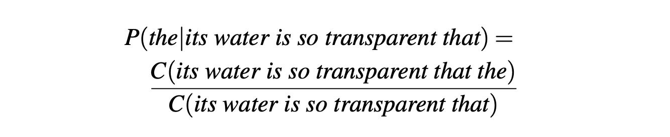
We call this ratio the relative frequency. The probability of a whole sequence is given by the chain rule of probabilities:

\[P(w_1, ..., w_N) = \prod_{k=1}^N (w_k \mid w_{k-1})\]

This approach seems logic, but the longer the sequence, the most likely it will be that we encounter 0’s, hence bringing the probability of the whole sequence at 0.

What solutions can we apply?

smoothing: redistribute the probability mass from observed to unobserved events (e.g Laplace smoothing, Add-k smoothing)
backoff: explained below

1. N-gram language model

But one of the most popular solution is the n-gram model. The idea behind the n-gram model is to truncate the word history to the last 2, 3, 4 or 5 words, and therefore approximate the history of the word:

\[P(w_i \mid h) = P(w_i \mid w_{i-n+1}, ..., w_{i-1})\]

We take \(n\) as being 1 (unigram), 2 (bigram), 3 (trigram)…

Let us now discuss some practical implementation tricks:

we compute the log of the probabilities, rather than the probabilities themselves (to avoid floating point approximation to 0)
for the first word of a sequence, we need to define pseudo-words as being the first 2 missing words for the trigram: \(P(I \mid <s><s>)\)

With N-grams, it is possible that we encounter unseen N-grams in prediction. There is a technique called backoff that states that if we miss the trigram evidence, we use the bigram instead, and if we miss the bigram evidence, we use the unigram instead…

Another approach is linear interpolate, where we combine different order n-grams by linearly interpolating all the models:

\[P(w_n \mid w_{n-2} w_{n-1}) = \lambda_1 P(w_n \mid w_{n−2} w_{n−1}) + \lambda_2 P(w_n \mid w_{n−1}) + \lambda_3 P(w_n)\]

2. Language models evaluation metrics

There are 2 types of evaluation metrics for language models:

extrinsic evaluation, for which we embed the language model in an application and see by which factor the performance is improved
intrinsic evaluation that measures the quality of a model independent of any application

Extrinsic evaluations are often heavy to implement. Hence, when focusing on intrinsic evaluations, we:

split the dataset/corpus into train and test (and development set if needed)
learn transition probabilities from the trainig set
use the perplexity metric to evaluate the language model on the test set

We could also use the raw probabilities to evaluate the language model, but the perpeplixity is defined as the inverse probability of the test set, normalized by the number of words. For example, for a bi-gram model, the perpeplexity (noted PP) is defined as:

\[PP(W) = \sqrt[^N]{ \prod_{i=1}^{N} \frac{1}{P(w_i \mid w_{i-1})}}\]

The lower the perplexity, the better

3. Limits of language models

Language models are trained on a closed vocabulary. Hence, when a new unknown word is met, it is said to be Out of Vocabulary (OOV).

4. Deep learning language models

More recently in Natural Language Processing, neural network-based language models have become more and more popular. Word embeddings project words into a continuous space \(R^d\), and respect topological properties (semantics and morpho-syntaxic).

Recurrent neural networks and LSTMs are natural candidates when learning such language models.

Decoding

The training is now done. The final step to cover is the decoding, i.e. the predictions to make when we collect audio features and want to produce transcript.

We need to find:

\[W^{\star} = argmax_W P(X \mid W) P(W) I^{\mid W \mid}\]

However, exploring the whole spact, especially since the Language Model \(P(W)\) has a really large scale factor, can be incredibly long.

One of the solutions is to explore the Beam Search. The Beam Search algorithm greatly reduces the scale factor within a language model (whether N-gram based or Neural-network-based). In Beam Search, we:

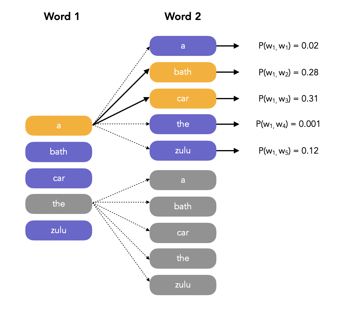
identify the probability of each word in the vocabulary for the first position, and keep the top K ones (K is called the Beam width)
for each of the K words, we compute the conditional probability of observing each of the second words of the vocabulary
among all produced probabilities, we keep only the top K ones
and we move on to the third word…

Let us illustrate this process the following way. We want to evaluate the sequence that is the most likely. We first compute the probability of the different words of the vocabulary to be the starting word of the sentence:

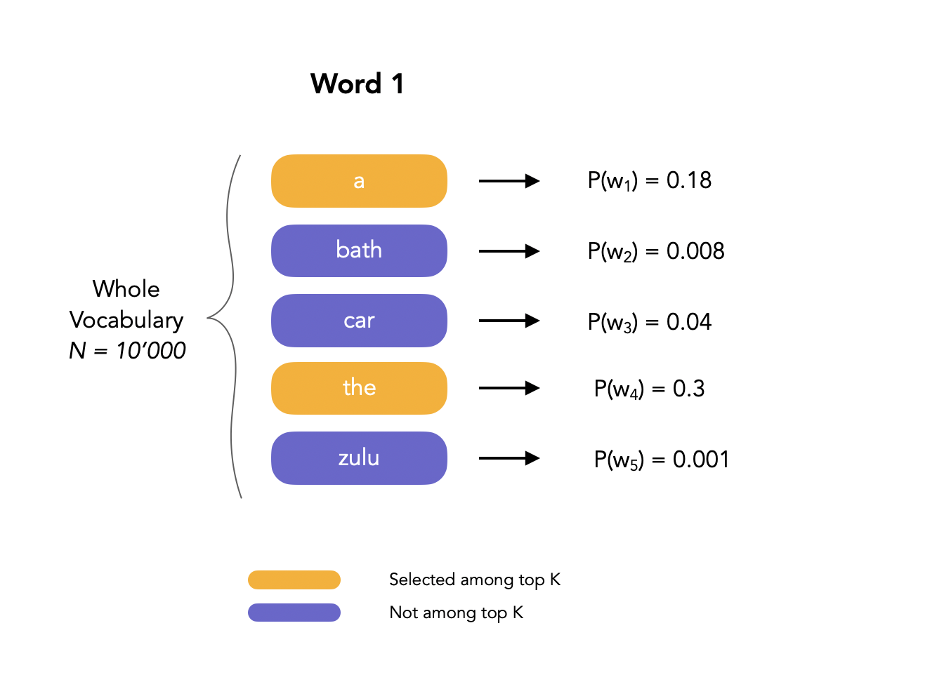
Here, we fix the beam width to 2, meaning that we only select the 2 most likely words to start with. Then, we move on to the next word, and compute the probability of observing it using conditional probability in the language model: \(P(w_2, w_1 \mid W) = P(w_1 \mid W) P(w_2 \mid w_1, W)\). We might see that a potential candidate, e.g. “The”, when selecting the top 2 candidates second words among all possible words, is not a possible path anymore. In that case, we narrow the search, since we know that the first must must be “a”.

And so on… Another approach to decoding is the Weighted Finite State Transducers (I’ll make an article on that).

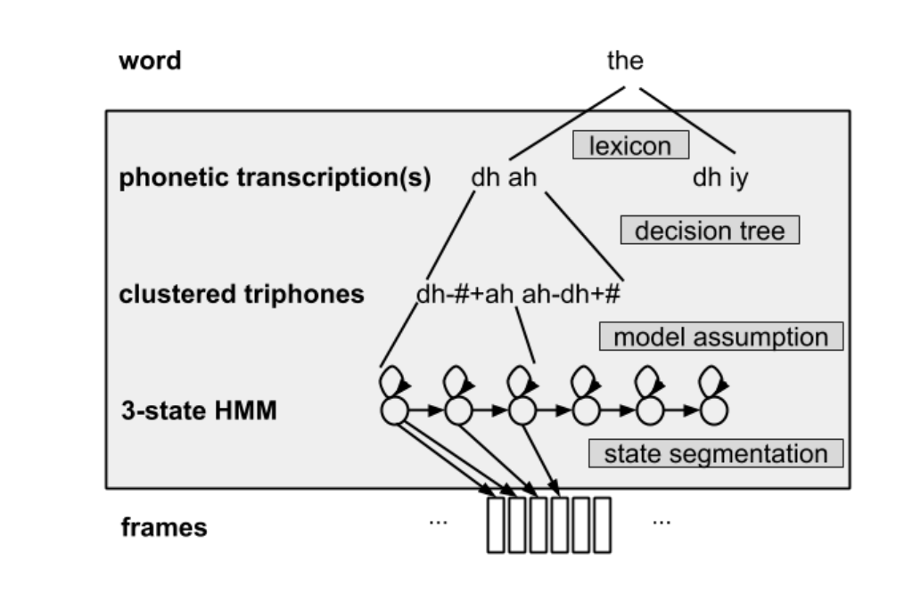
Summary of the ASR pipeline

In their paper “Word Embeddings for Speech Recognition”, Samy Bengio and Georg Heigold present a good summary of a modern ASR architecture:

Words are represented through lexicons as phonemes
Typically, for context, we cluster triphones
We then assume that these triphones states were in fact HMM states
And the the observations each HMM state generates are produced by DNNs or GMMs

End-to-end approach

Alright, this article is already long, but we’re almost done. So far, we mostly covered historical statistical approaches. These approaches work very well. However, most recent papers and implementations focus on end-to-end approaches, where:

we encode \(X\) as a sequence of contexts \(C\)
we decode \(C\) into a sequence of words \(W\)

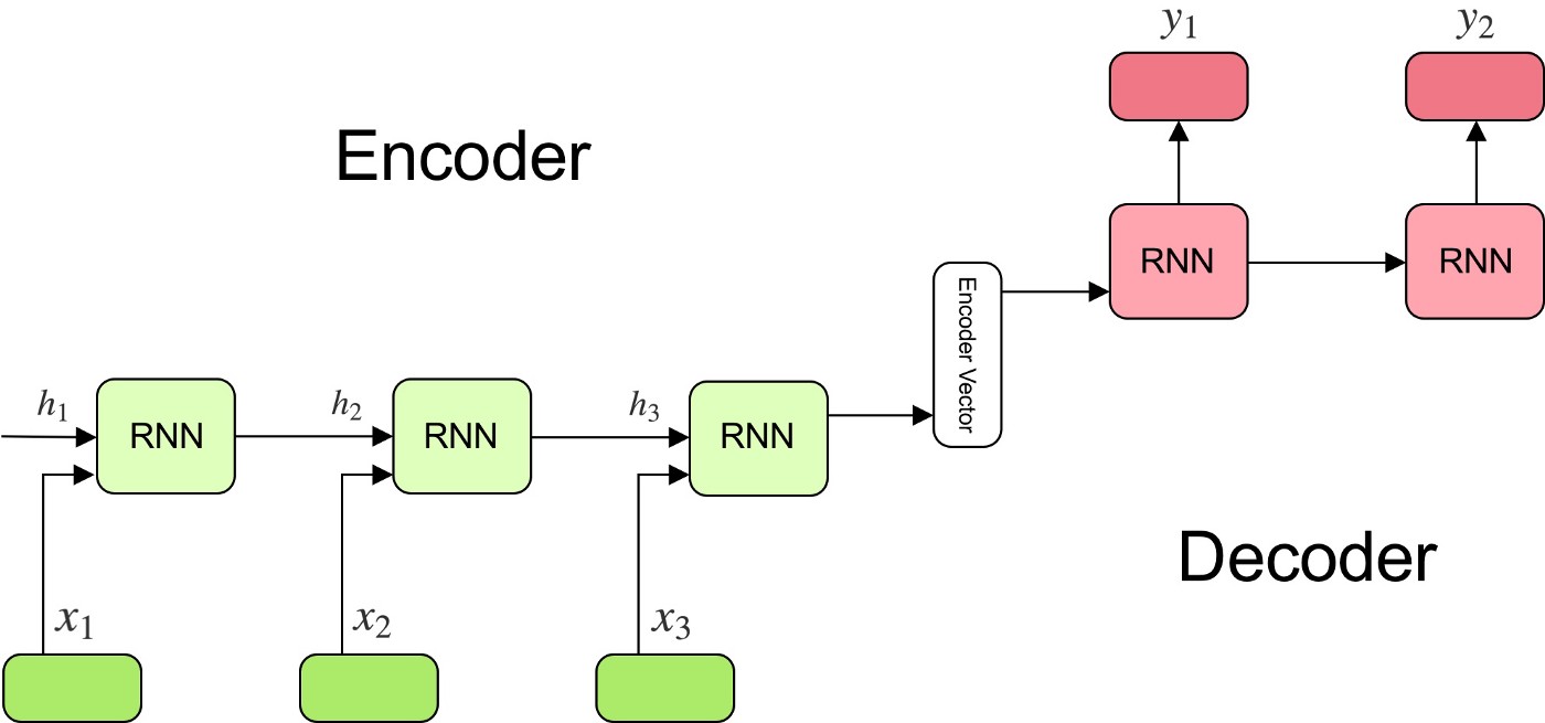
These approaches, also called encoder-decoder, are part of sequence-to-sequence models. Sequence to sequence models learn to map a sequence of inputs to a sequence of outputs, even though their length might differ. This is widely used in Machine Translation for example.

As illustrated below, the Encoder reduces the input sequence to a encoder vector through a stack of RNNs, and the decoder vector uses this vector as an input.

I will write more about End-to-end models in another article.

Conclusion

This is all for this quite long introduction to automatic speech recognition. After a brief introduction to speech production, we covered historical approaches to speech recognition with HMM-GMM and HMM-DNN approaches. We also mentioned the more recent end-to-end approaches. If you want to improve this article or have a question, feel free to leave a comment below :)

References:

Introduction to Automatic Speech Recognition (ASR)

Maël Fabien

Introduction to ASR

What is ASR?

How is speech produced?

Breaking down words

Evaluation metrics

Statistical historical approach to ASR

Feature extraction \(X\)

Acoustic model

1. HMM-GMM acoustic Model

2. HMM-DNN acoustic model

3. HMM-DNN vs. HMM-GMM

4. End-to-end models

Pronunciation

Language Modeling

1. N-gram language model

2. Language models evaluation metrics

3. Limits of language models

4. Deep learning language models

Decoding

Summary of the ASR pipeline

End-to-end approach

Conclusion