Disrupting Resilient criminal networks through data analysis

In this article, I will re-implement and discuss the paper: “Disrupting resilient criminal networks through data analysis: the case of Sicilian Mafia” by Lucia Cavallaro and Annamaria Ficara and Pasquale De Meo and Giacomo Fiumara and Salvatore Catanese and Ovidiu Bagdasar and Antonio Liotta.

They published real world data, and I will also explore it on my side. The Github of the project with the code and data can be found here.

Background

This study focuses on the structure of the Sicilian Mafia as a criminal network. The whole network is made of sub-groups referred as families.

The authors have built two real-world anonymized datasets, based on raw data derived from juridical acts, relating to a Mafia gang that operated in Sicily (Italy) during the first decade of 2000s:

• a dataset of phonecalls
• a dataset of physical meetings

The authors apply techniques of Social Network Analysis (SNA) to identify the best technique to disrupt the network (which member to arrest, in what order…).

Strategies to disrupt networks rely on:

• human capital, a strategy in which we investigate the resources possessed by actors of a network
• social capital, a strategy in which we arrest actors with the largest social link in the network (e.g brokers that are bridges between two markets)

In social capital, the removal of the actors with the largest betweenness centrality tends to be the best technique. After disruption, the network might still be exist. We talk about network resilience. This is what this paper focuses on.

Data

For this part, I won’t cover too much what the authors did and I will explore this dataset using my approach/visualization. I will rely on networkx (quite common), but also on Nx_altair, a library (which I think isn’t maintained anymore) that mixes Altair and Networkx.

import numpy as np
import pandas as pd

# Visualization
import matplotlib.pyplot as plt
import altair as alt

# Networks
import networkx as nx
import nx_altair as nxa
from networkx.algorithms.community import greedy_modularity_communities

We will first focus on the physical meeting dataset and build the corresponding graph:

file = open('Datasets/Montagna_meetings_edgelist.csv', 'r')

G = nx.Graph()
for row in file:
    r = row.split()
    n1, n2, w = int(r[0]), int(r[1]), int(r[2])
    G.add_node(n1)
    G.add_node(n2)
    G.nodes[n1]['id'] = n1
    G.nodes[n2]['id'] = n2
    G.add_edge(n1, n2)
    G.edges[(n1,n2)]['weight']=w
    G.edges[(n1,n2)]['method']='meetings'

We attributed a weight to each edge based on how frequently two nodes met.

Now, let’s make a first plot of the network and the meetings between the nodes.

pos = nx.spring_layout(G)

chart = nxa.draw_networkx(
    G=G,
    pos=pos,
    width='weight:N',
    node_tooltip=['id:N']
).properties(title="Sicilian Mafia physical meetings", height=500, width=500
).interactive()

chart

We can now try to discribe a bit further the network (number of nodes, edges, degree…):

c_degree = nx.degree_centrality(G)
c_degree = list(c_degree.values())
c = list(greedy_modularity_communities(G))

nb_nodes = len(list(G.nodes()))
nb_edges = len(list(G.edges()))
degrees = list(dict(G.degree()).values())
avg_degree = np.mean(degrees)
median_degree = np.median(degrees)
max_degree = np.max(degrees)        
min_degree = np.min(degrees) 
avg_centrality = np.mean(c_degree) 
min_centrality = np.min(c_degree) 
max_centrality = np.max(c_degree) 
median_centrality = np.median(c_degree) 

print("Number of nodes: ", nb_nodes)
print("Number of edges: ", nb_edges)
print("Average degree: ", avg_degree)
print("Median degree: ", median_degree)
print("Max degree: ", max_degree)
print("Min degree: ", min_degree)
print("Average centrality: ", avg_centrality)
print("Median centrality: ", median_centrality)
print("Max centrality: ", max_centrality)
print("Min centrality: ", min_centrality)

It heads the following:

Number of nodes:  101
Number of edges:  256
Average degree:  5.069306930693069
Median degree:  3.0
Max degree:  24
Min degree:  1
Average centrality:  0.050693069306930696
Median centrality:  0.03
Max centrality:  0.24
Min centrality:  0.01

On average, each person is connected to 5 other (which is quite high). There seems to be a least one person with a large centrality since this person has 24 edges.

We can now look at the distribution of the degrees:

hist = alt.Chart(pd.DataFrame(degrees, columns=['Degrees'])).mark_bar().encode(
    alt.X("Degrees:Q", bin=alt.Bin(maxbins=25)),
    y='count()').properties(title="Degree Distribution", height=300, width=500)

hist

It is much closer to a Barabasi-Albert model distribution, meaning that the network has strong signs of preferential attachment.

The two datasets have 47 nodes in common, so we can plot them together:

file = open('Datasets/Montagna_phonecalls_edgelist.csv', 'r')

for row in file:
    r = row.split()
    n1, n2, w = int(r[0]), int(r[1]), int(r[2])
    G.add_node(n1)
    G.add_node(n2)
    G.nodes[n1]['id'] = n1
    G.nodes[n2]['id'] = n2
    G.add_edge(n1, n2)
    G.edges[(n1,n2)]['weight']=w
    G.edges[(n1,n2)]['method']='phonecalls'

pos = nx.spring_layout(G)

chart = nxa.draw_networkx(
    G=G,
    pos=pos,
    width='weight:N'
).properties(title="Sicilian Mafia all meetings", height=500, width=500
).interactive()

chart

Now, we can try to display nodes in a different color if their betweenness centrality is above a certain threshold (here, 0.15). We identify three central nodes, which also look like the main information bottleneck in the graph. I do not have much information on these nodes, but we can easily suppose that these people play a key role in their communities. Zoom in the graph to see more details:

c_degree = nx.betweenness_centrality(G)
c_degree = list(c_degree.values())

chart = nxa.draw_networkx(
    G=G,
    pos=nx.spring_layout(G),
    width='weight:N',
    node_tooltip=['id','is_central']
)

edges = chart.layer[0].properties(height=500, width=500)
nodes = chart.layer[1].properties(height=500, width=500)

nodes = nodes.encode(
    fill='is_central:N',
    color='is_central:N'
).properties(
    height=500, width=500, title="Centrality"
)

central = (edges+nodes).interactive()

central

We can focus on running a simple community detection algorithm. We use the greedy modularity algorithm from NetworkX:

c = list(greedy_modularity_communities(G))

for n in G.nodes():
    if n in list(c[0]):
        G.nodes[n]['community'] = '0'
    elif n in list(c[1]):
        G.nodes[n]['community'] = '1'
    elif n in list(c[2]):
        G.nodes[n]['community'] = '2'
    elif n in list(c[3]):
        G.nodes[n]['community'] = '3'
    elif n in list(c[4]):
        G.nodes[n]['community'] = '4'
    elif n in list(c[5]):
        G.nodes[n]['community'] = '5'
    elif n in list(c[6]):
        G.nodes[n]['community'] = '6'
    elif n in list(c[7]):
        G.nodes[n]['community'] = '7'
    elif n in list(c[8]):
        G.nodes[n]['community'] = '8'

chart = nxa.draw_networkx(
    G=G,
    pos=nx.spring_layout(G),
    width='weight:N',
    node_tooltip=['id','community']
)

edges = chart.layer[0].properties(height=500, width=500)
nodes = chart.layer[1].properties(height=500, width=500)

nodes = nodes.encode(
    fill='community:N',
    color='community:N'
).properties(
    height=500, width=500, title="Community"
)

community = (edges+nodes).interactive()

community

8 communities have been detected, and the communities detected appear in various colors.

Network Disruption

As we have seen, there are some key players, and communities that are larger than others. When disruption a criminal network,it is therefore important to arrest the right persons and avoid the network resilience.

The authors use a metric to measure the network resilience:

\[\rho = 1 - \mid \frac{LCC_{i}(G_i) - LCC_{0}(G_0)} {LCC_{0}(G_0)} \mid\]

Where \(LCC\) is the Largest Connected Component, a measure of the total number of nodes of the largest connected component. A connected component of an undirected graph is a subgraph in which any two vertices are connected to each other by paths, and which is connected to no additional vertices outside of this component. In brief, this metric tracks by how much we damaged the LCC of the network by removing one or few nodes.

In the whole graph, the connected components can be computed as such:

for x in nx.connected_components(G):
    print(x)

{0, 1, 2}
{3, 4, 5, 6, 7, 8, 9, 10, 11, 12, 13, 14, 15, 18, 19, 20, 21, 22, 23, 24, 25, 26, 27, 28, 29, 30, 31, 32, 33, 34, 35, 36, 37, 38, 39, 40, 41, 42, 43, 44, 45, 46, 47, 48, 49, 50, 51, 52, 53, 54, 55, 56, 57, 58, 59, 60, 61, 62, 63, 64, 65, 66, 67, 68, 69, 70, 71, 72, 75, 76, 77, 78, 79, 80, 81, 82, 83, 84, 85, 86, 87, 88, 89, 90, 91, 92, 93, 94, 95, 96, 97, 98, 99, 100, 101, 102, 103, 104, 105, 108, 109, 110, 111, 112, 113, 114, 115, 116, 117, 118, 119, 120, 121, 122, 123, 124, 125, 126, 127, 128, 129, 130, 131, 132, 133, 134, 135, 136, 137, 138, 139, 140, 141, 142, 143, 144, 145, 146, 147, 148, 149, 150, 151, 152, 153}
{16, 17}
{73, 74}
{106, 107}

Just like we can visually observe, there is one major connected component. We can see the number of nodes of each sub-graph using:

for x in nx.connected_components(G):
    print(nx.number_of_nodes(G.subgraph(x)))

3
145
2
2
2

The LCC is therefore the max of those, which is 145.

We can therefore define a function to look for the LCC size:

def lcc_size(graph):

    compsize = []
    for c in nx.connected_components(graph):
        compsize.append(nx.number_of_nodes(graph.subgraph(c)))
    return max(compsize)

The idea behind the metric is to iteratively remove:

• either the node with the highest collective influence, in a sequential manner
• or the top 5 nodes with the highest collective influence, in a “block” manner

And see how the metric evolves. If you want to learn more about collective influence, make sure to check this article.

To gradually remove the nodes (in a sequential manner), the authors propose a function:

import array
import copy

toremove = array.array('i', [])
nrem = 5
names = ['id', 'data']
formats = ['int32', 'int32']
dtype = dict(names=names, formats=formats)

def disruption_sequence(Graph, weight=None):

    Gor = copy.deepcopy(Graph)
    lccinit = lcc_size(Graph) 
    dflcc = pd.DataFrame()
    dflccvar = pd.DataFrame()

    dictx = dict()
    dicty = dict()
    kiter = 0
    toremove = array.array('i', [])
    
    while Gor.number_of_nodes() > nrem:

        i = 0

        while i < nrem:
            if Gor.number_of_nodes() <= nrem:
                break

            toremove = array.array('i', [])
            dictx[kiter] = lcc_size(Gor)
            dicty[kiter] = 1 - (abs((lcc_size(Gor) - lccinit) / lccinit))
            toremove = collective_influence_centality(Gor, toremove, weight=weight)
            
            Gor.remove_node(toremove[0])
            toremove.pop(0)
            kiter += 1
            i += 1
            
    dflcc['No'] = list(dictx.keys())
    dflccvar['No'] = dflcc['No']
    dflcc['centrality'] = list(dictx.values())
    dflccvar['centrality'] = list(dicty.values())
    
    return dflcc, dflccvar

dflcc, dflccvar = disruption_sequence(G)

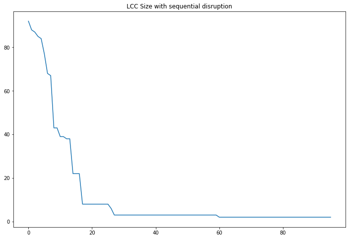
We store the LCC and the score of the network given the sequential disruption. We can then plot the result:

plt.figure(figsize=(12,8))
plt.plot(dflcc['No'], dflcc['centrality'])
plt.title("LCC Size with sequential disruption")
plt.show()

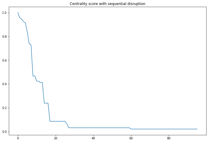
We can also plot the score described above:

plt.figure(figsize=(12,8))
plt.plot(dflccvar['No'], dflccvar['centrality'])
plt.title("Centrality score with sequential disruption")
plt.show()

For the block-removal, one can simply remove 5 nodes before re-computing the collective influence candidates to remove:

def disruption_block(Graph, weight=None):

    Gor = copy.deepcopy(Graph)
    lccinit = lcc_size(Graph) 
    dflcc = pd.DataFrame()
    dflccvar = pd.DataFrame()

    dictx = dict()
    dicty = dict()
    kiter = 0
    toremove = array.array('i', [])

    while Gor.number_of_nodes() > nrem:
        i = 0

        toremove = array.array('i', [])
        dictx[kiter] = lcc_size(Gor)
        dicty[kiter] = 1 - (abs((lcc_size(Gor) - lccinit) / lccinit))
        toremove = collective_influence_centality(Gor, toremove, weight=weight)
        
        while i < nrem:
            if Gor.number_of_nodes() <= nrem:
                break
            Gor.remove_node(toremove[0])
            toremove.pop(0)
            kiter += 1
            i += 1
    
    dflcc['No'] = list(dictx.keys())
    dflccvar['No'] = dflcc['No']
    dflcc['centrality'] = list(dictx.values())
    dflccvar['centrality'] = list(dicty.values())
    
    return dflcc, dflccvar

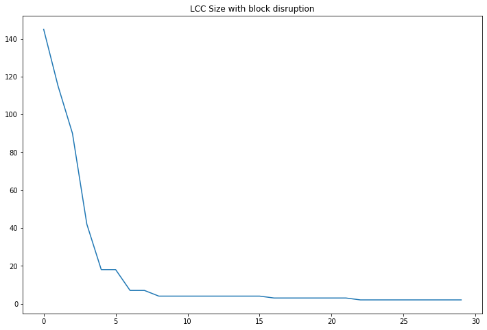
And as before, we can compute the LCC and the score with the number of iterations:

dflcc, dflccvar = disruption_block(G)
plt.figure(figsize=(12,8))
plt.plot(dflcc['centrality'])
plt.title("LCC Size with block disruption")
plt.show()

plt.figure(figsize=(12,8))
plt.plot(dflccvar['centrality'])
plt.title("Centrality score with block disruption")
plt.show()

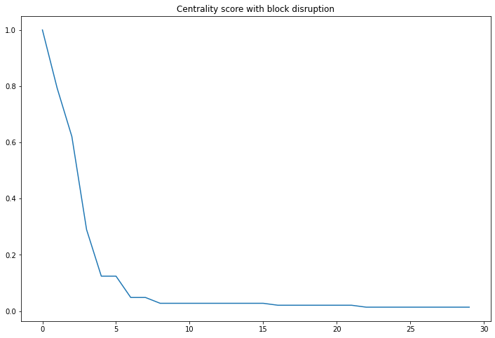
Note, the results are quite similar in terms when you compare the number of persons who had to be arrested.

Discussion

The authors discuss that betweenness centrality is the best metric to apply (better than collective influence), given the focus it has on information bottleneck. 5% of the network is often responsible for more than 70% of the information (and this is real-world data !).

The dataset provided is static (meaning that we do not know how the network will react to a disruption). Overall, the metric provided is interesting, and this kind of approach could be explored in criminal network investigations.