Large Scale Kernel Methods

Kernel methods such as Kernel SVM have some major issues regarding scalability. You might have encountered some issues when trying to apply RBF Kernel SVMs on a large amount of data.

Two major algorithms allow to easily scale Kernel methods :

• Random Kernel features
• Nyström approximation

We’ll recall what Kernel methods are, and cover both methods.

For what comes next, you might want to open a Jupyter Notebook and import the following packages :

import numpy as np
from scipy import linalg
import matplotlib.pyplot as plt
plt.style.use('ggplot')

from sklearn.metrics import accuracy_score
from sklearn.model_selection import train_test_split
from sklearn.preprocessing import StandardScaler
from sklearn.datasets import load_svmlight_file
from sklearn.datasets import make_classification

from sklearn.svm import SVC, LinearSVC
from time import time

from scipy.sparse.linalg import svds
from scipy.linalg import svd
from scipy.sparse import csc_matrix
from numpy.linalg import multi_dot
from numpy.linalg import norm

from math import pi

I. Recall on Kernel Methods

SVM Classifier

We’ll consider a binary classification framework. Suppose we have training observations \(X_1, ..., X_n \subset R^p\) , and training labels \(y_1, ..., y_n ∈ {-1,1}\) .

We can define the non-linearly separable SVM framework as follows :

\[min_{w ∈ R^p, b ∈ R, \epsilon ∈ R^n} \frac {1} {2} { {\mid \mid w \mid \mid }_2 }^2 + C \sum_i {\epsilon}_i\]

subject to :

\[y_i ( w^T X + b) ≥ 1 - {\epsilon_i}, i = 1 ... n\] \[{\epsilon_i} ≥ 0, i = 1 ... n\]

We can rewrite this as a dual problem using a Lagrange formulation :

\[max_{\alpha ∈ R^n} {\sum}_i {\alpha}_i - \frac {1} {2} {\alpha}_i {\alpha}_j y_i y_j {X_i}^T X_j\]

subject to :

\[0 ≤ {\alpha}_i ≤ C, i = 1 ... n\] \[{\epsilon}_i , i = 1 ... n\]

The binary classifier is : \(f(x) = sign( \sum_i {\alpha}_i y_i {X_i}^T X_i )\)

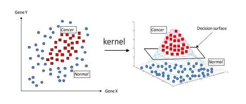
The kernel trick

A symmetric function \(K : χ \times χ → R\) is a kernel if there exists a mapping function \(\phi : χ → R\) from the instance space \(χ\) to a Hilbert space \(H\) such that \(K\) can be written as an inner product in \(H\) :

\[K(X, X') = < \phi(X), \phi(X') >\]

The Kernel trick can be visualized as a projection of an initial problem with a complex decision frontier into feature space in which the decision frontier is way easier and faster to build.

The Kernel SVM can be expressed as :

\[max_{\alpha ∈ R^n} {\sum}_i {\alpha}_i - \frac {1} {2} {\alpha}_i {\alpha}_j y_i y_j K ({X_i}^T X_j)\]

subject to :

\[0 ≤ {\alpha}_i ≤ C, i = 1 ... n\] \[\sum_i {\alpha}_i y_i = 0, i = 1 ... n\]

The binary classifier is : \(f(x) = sign( \sum_i {\alpha}_i y_i K({X_i}^T X_i ))\)

Types of kernels

What types of kernels can be used?

• Linear kernel : \(K(X,X') = X^T X'\)
• Polynomial kernel : \(K(X,X') = (X^T X' + c)^d\)
• Gaussian RBF kernel : \(K(X,X') = exp( - \gamma { { \mid \mid X - X' \mid \mid}_2 }^2 )\)
• Laplace RBF kernel : \(K(X,X') = exp( - \gamma { \mid \mid X - X' \mid \mid}_1 )\)

Kernels allow non-linear variants for many linear machine learning algorithms :

• SVM
• Ridge Regression
• PCA
• K-Means
• and others …

In Python

First of all, we’ll generate some articifical data :

X, y = make_classification(n_samples=100000)
X_train, X_test, y_train, y_test = train_test_split(X, y, random_state=42)

We now have 75’000 training data and 25’000 test data. We first scale the data.

scaler = StandardScaler()
X_train = scaler.fit_transform(X_train)
X_test = scaler.transform(X_test)

n1, p = X_train.shape
n2 = X_test.shape[0]

print("Training samples :", n1)
print("Test samples:", n2)
print("Features:", p)

Linear Support Vector Classifier

# Train
t0 = time()
clf_lin = LinearSVC(dual=False)
clf_lin.fit(X_train, y_train)
print("done in %0.3fs" % (time() - t0))

done in 0.334s

# Test
t1 = time()
timing_linear = time() - t1
y_pred = clf_lin.predict(X_test)
print("done in %0.3fs" % (time() - t1))

done in 0.016s

# Accuracy
accuracy_linear = accuracy_score(y_pred, y_test)
print("classification accuracy: %0.3f" % accuracy_linear)

classification accuracy: 0.868

Gaussian RBF Kernel Support Vector Classifier

# Train
t0 = time()
clf = SVC(kernel='rbf')
clf.fit(X_train, y_train)
print("done in %0.3fs" % (time() - t0))

done in 375.102s

# Test
t1 = time()
y_pred = clf.predict(X_test)
timing_kernel = time() - t1
print("done in %0.3fs" % (time() - t1))

done in 40.148s

# Accuracy
accuracy_kernel = accuracy_score(y_pred, y_test)
print("classification accuracy: %0.3f" % accuracy_kernel)

classification accuracy: 0.891

The classification accuracy improves when we use the Gaussian RBF. However, the training and prediction times are now much longer.

II. Limits of Kernel methods

Kernel methods rely on Gram Matrix : \(G ∈ R^{n \times n}\)

The Gram martix has the following form :

\[\begin{pmatrix} K(X_1, X_1) & K(X_1, X_2) & .. & K(X_1, X_n) \\ ... & ... & ... & ... \\ K(X_n, X_1) & K(X_n, X_2) & .. & K(X_n, X_n) \end{pmatrix}\]

The complexity of the kernel evaluation in the training is \(O(n^2)\).

The complexity of the prediction is \(O(n)\). Overall, this becomes infeasible for large \(n\).

We’ll now cover the two most common ways to overcome this problem :

• Random Kernel features: approximate the kernel function
• Nyström approximation: approximate the Gram matrix

III. Random Kernel features

Principle

If we don’t apply the Kernel SVM, the problem can be expressed the following way :

\[min_{w,b} \frac {1} {2} { { \mid \mid w \mid \mid }_2 }^2 + C \sum_i [ y_i (W^T \phi(X) + b)]_+\]

where \([a]_+ = max(0, 1-a)\) is the hingle loss function.

Usually, \(\phi(X)\) is unknown and potentially infinite-dimensional, and implies \(O(n^2)\) or \(O(n^3)\) complexity.

The idea of Randon Kernel Features is to find a finite dimensional feature map \(\hat{ \phi } (X) ∈ R^c\) such that :

\[K(X, X') ≈ < \hat{\phi}(X), \hat{\phi}(X') >\]

We should be able to solve the primal form to get \(w\) and \(b\), and use the approximated kernel in a binary classification : \(f(x) = sign (w^T \hat{ \phi } (X) + b)\) .

Botchner’s Theorem

A kernel is said to be shift-invariant if and only if for any \(a ∈ R^p\) and any \((x,x') ∈ R^p \times R^p\) :

\[K (x-a, x'-a) = K (x, x')\] \[K (x, x') = K (x-x') = K ( \Delta)\]

We’ll consider shift-invariant kernels \(K (x-x') = K ( \Delta)\) (Gaussian RBF and Laplace RBF) in order to apply Bochner’s theorem. This theorem states that a continuous shift-invariant kernel is positive definite if and only if \(K ( \Delta)\) is the Fourier transform of a non-negative probability measure.

It can be shown (the demonstration is skipped for this article) that :

\[K (x, x') = E_{w \sim P, b \sim U[0, 2 \pi]} [ \sqrt{2} cos (w^T x + b) \sqrt{2} cos (w^T x' + b)]\]

The kernel is an infinite sum since we consider all values of \(w\) and \(b\). The kernel has, therefore, an infinite dimension.

Kernel approximation

A usual technique to approximate such problem is random sampling! If we know the distributions of \(w\) and \(b\), by Monte-Carlo principle, we’ll approach the result of the RBF Kernel!

The distributions are the following :

• \(b\) follows a uniform distribution : \(b \sim U[0, 2 \pi]\)
• \(w\) follows \(P (w)\) the scaled fourier transform of \(K(\Delta)\)

If the Kernel is Gaussian, \(P\) is Gaussian itself : \(P \sim N(0, 2 \gamma)\), where the default value of \(\gamma\) is \(\frac {1} {p}\) , \(p\) being the number of features . If the Kernel is Laplacian, \(P\) is a Cauchy distribution.

Pseudo-Code

1. Set the number of random kernel features to \(c\)
2. Draw \(w_1, ..., w_c \sim P(w)\) and \(b_1, ..., b_c \sim U [0, 2 \pi]\)
3. Map training points \(x_1, ..., x_n ∈ R^p\) to their random kernel features \(\hat{\phi} (X_1), ..., \hat{\phi} (X_n) ∈ R^c\) where \(\hat{\phi} (X_i) = \sqrt{ \frac {2} {c} } cos ( {w_i}^T X + b_j), j ∈ [1, ... , c]\). \(c\) is present in the fraction to create a mean.
4. Train a linear model (such as Linear SVM) on transformed data \(\hat{\phi} (X_1), ..., \hat{\phi} (X_n) ∈ R^c\)

In other words, to speed up the whole training process and get results that tend to be similar to RBF kernel, we pre-process the data and apply a linear SVM on top. It can be shown that this approximation will converge to the RBF Kernel.

Moreover, the kernel approximation error uniformly decreases in \(O( \sqrt { \frac {1} {c} } )\).

In Python

Let’s define the random_features function that will return the modified training data according to the pseudo-code above :

def random_features(X_train, X_test, gamma, c=300, seed=42):
    rng = np.random.RandomState(seed)
    n_samples, n_features = X_train.shape

    W = np.random.normal(0, np.sqrt(2*gamma), (n_features, c))
    b = np.random.uniform(0, 2*pi, (1,c))

    X_new_train = np.sqrt(2/n_features) * np.cos(np.dot(X_train, W) + b)
    X_new_test = np.sqrt(2/n_features) * np.cos(np.dot(X_test, W) + b)

    return X_new_train, X_new_test

As defined above, the default value of \(\gamma\) is \(\frac {1} {p}\) :

n_samples, n_features = X_train.shape
gamma = 1. / n_features

Then, modify the input data using the random kernel feature :

Z_train, Z_test = random_features(X_train, X_test, gamma, c=800)

We’ll now assess the efficiency of this technique :

t0 = time()
clf = LinearSVC(dual=False)
clf.fit(Z_train, y_train)
print("done in %0.3fs" % (time() - t0))

done in 39.525s

t1 = time()
accuracy = clf.score(Z_test, y_test)
print("done in %0.3fs" % (time() - t1))
print("classification accuracy: %0.3f" % accuracy)

done in 0.089s classification accuracy: 0.881

The classification is very close to the one achieved by RBF. However, the computation time has been divided by 10 overall.

IV. Nyström Approximation

The essence of the Nyström approximation is to offer an approximation of the Gram matrix involved in the computation by spectral decomposition.

Let \(G ∈ R^{n \times n}\) be a Gram matrix such that \(G_{i,j} = K(X_i, X_j)\) . When \(n\) gets large, we want to approximate \(G\) with a lower rank matrix.

Spectral decomposition

Recall that the spectral decomposition is defined as : \(G = U Λ U^T\) where :

• \(U = [u_1, ... , u_n]^T ∈ R^{n \times n}\) a set of eigenvectors
• \(Λ = diag( \lambda_1, ..., \lambda_n)\) a set of eigenvalues

The best rank-k approximation \(G_k\) of \(G\) is given by \(G_k = U_k Λ_k {U_k}^T\) where :

• \[U_k ∈ R^{n \times k}\]
• \[Λ = diag( \lambda_1, ..., \lambda_k)\]

We only keep the \(k^{th}\) largest eigenvalues.

Limitations and motivation

However, in our case, this is useless. We need to construct \(G\) in \(O(n^2)\) time and compute its \(k^{th}\) best rank approximation in \(O(n^2)\) to \(O(n^3)\) depending on the value of \(k\).

Our goal is therefore to find a good approximation \(\hat {G_k}\) of \(G_k\) in \(O(n)\) time.

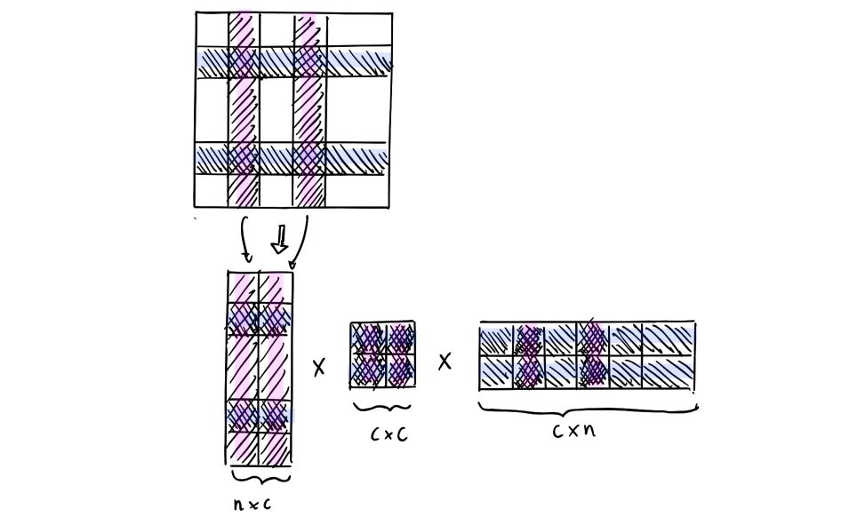
For this reason, we introduce the Nyström approximation :

\(\hat{G_k} = C W^+ C^T\) where :

• \[C ∈ R^{n \times c}\]
• \[W ∈ R^{c \times c}\]
• \(W^+\) the Moore-Penrose (pseudo) inverse

This decomposition might seem a bit weird since we sample the columns and the rows of the Gram matrix. First of all, it can only be applied to Gram matrices, not to any kind of matrix. Suppose that we take a look at a matrix of distances between different cities. Would you need all the distances between all the cities to provide a pretty accurate estimate of the distance between 2 cities? Well, there’s definitely some pieces of information that have a little importance and bring few additional precision. This is exactly what we’re doing here on the Gram matrix.

Pseudo-code

1. Sample a set \(I\) of \(c\) indices uniformly in \({1,...,n}\)
2. Compute \(c ∈ R^{n \times c}\) with \(c_{ij} = K(X_i, X_j), i ∈ {1,...,n}, j ∈ I\)
3. Form a matrix \(W ∈ R^{c \times c}\) with \(W_{ij} = K(X_i, X_j), i, j ∈ I\)
4. Compute \(W_k ∈ R^{c \times c}\) the best rank-k approximation of \(W\)
5. Compute the final rank-k matrix of G : \(\hat{G_k} = C {W_k}^+ C^T ∈ R^{n \times n}\)

The complexity is \(O(c^3 + nck)\) . The convergence of this approximation has also been demonstrated.

In Python

Define the function corresponding to the Nyström approximation :

def nystrom(X_train, X_test, gamma, c=500, k=200, seed=44):

    rng = np.random.RandomState(seed)
    n_samples = X_train.shape[0]
    idx = rng.choice(n_samples, c)

    X_train_idx = X_train[idx, :]
    W = rbf_kernel(X_train_idx, X_train_idx, gamma=gamma)

    u, s, vt = linalg.svd(W, full_matrices=False)
    u = u[:,:k]
    s = s[:k]
    vt = vt[:k, :]

    M = np.dot(u, np.diag(1/np.sqrt(s)))

    C_train = rbf_kernel(X_train, X_train_idx, gamma=gamma)
    C_test = rbf_kernel(X_test, X_train_idx, gamma=gamma)

    X_new_train = np.dot(C_train, M)
    X_new_test = np.dot(C_test, M)

    return X_new_train, X_new_test

Modify the input data :

Z_train, Z_test = nystrom(X_train, X_test, gamma, c=500, k=300, seed=44)

Fit the model :

t0 = time()
clf = LinearSVC(dual=False)
clf.fit(Z_train, y_train)
print("done in %0.3fs" % (time() - t0))

done in 15.260s

And compute the accuracy :

t1 = time()
accuracy = clf.score(Z_test, y_test)
print("done in %0.3fs" % (time() - t1))
print("classification accuracy: %0.3f" % accuracy)

done in 0.021s classification accuracy: 0.886

The results are overall better than Linear SVC and random kernel features, and the computation time is way smaller.

V. Performance overview

In this section, we’ll compare the performances of the different versions of the classifier in terms of accuracy and computation time :

ranks = np.arange(20, 600, 50)
n_ranks = len(ranks)

timing_rkf = np.zeros(n_ranks)
timing_nystrom = np.zeros(n_ranks)
timing_linear = np.zeros(n_ranks)
timing_rbf = np.zeros(n_ranks)

accuracy_nystrom = np.zeros(n_ranks)
accuracy_rkf = np.zeros(n_ranks)
accuracy_linear = np.zeros(n_ranks)
accuracy_rbf = np.zeros(n_ranks)

print("Training SVMs for various values of c...")

for i, c in enumerate(ranks):

    print(i, c)

    ## Nystorm
    Z_ny_train, Z_ny_test = nystrom(X_train, X_test, gamma, c=c, k=300, seed=44)

    t0 = time()
    clf = LinearSVC(dual=False)
    clf.fit(Z_ny_train, y_train)
    accuracy_nystrom[i] = clf.score(Z_ny_test, y_test)
    timing_nystrom[i] = time() - t0

    ## Random Kernel Feature
    Z_rkf_train, Z_rkf_test = random_features(X_train, X_test, gamma, c=c, seed=44)
    t0 = time()
    clf = LinearSVC(dual=False)
    clf.fit(Z_rkf_train, y_train)
    accuracy_rkf[i] = clf.score(Z_rkf_test, y_test)
    timing_rkf[i] = time() - t0

    ## Linear
    t0 = time()
    clf = LinearSVC(dual=False)
    clf.fit(X_train, y_train)
    accuracy_linear[i] = clf.score(X_test, y_test)
    timing_linear[i] = time() - t0

    ## RBF
    t0 = time()
    clf = SVC(kernel='rbf')
    clf.fit(X_train, y_train)
    accuracy_rbf[i] = clf.score(X_test, y_test)
    timing_rbf[i] = time() - t0

If we plot the time and the accuracy depending on the number of features included, we obtain :

f, axes = plt.subplots(ncols=1, nrows=2, figsize=(10,6))
ax1, ax2 = axes.ravel()

ax1.plot(ranks-10, timing_nystrom, '-', label='Nystrom')
ax1.plot(ranks, timing_rkf, '-', label='RKF')
ax1.plot(ranks, timing_linear * np.ones(n_ranks), '-', label='LinearSVC')
ax1.plot(ranks, timing_kernel * np.ones(n_ranks), '-', label='RBF')

ax1.set_xlabel('Number of features')
ax1.set_ylabel('Time')
ax1.legend(loc='lower right')

ax2.plot(ranks-10, accuracy_nystrom, '-', label='Nystrom')
ax2.plot(ranks, accuracy_rkf, '-', label='RKF')
ax2.plot(ranks, accuracy_linear * np.ones(n_ranks), '-', label='LinearSVC')
ax2.plot(ranks, accuracy_kernel * np.ones(n_ranks), '-', label='RBF')
ax2.set_xlabel('Number of features')
ax2.set_ylabel('Accuracy')
ax2.legend(loc='lower right')
plt.tight_layout()
plt.show()

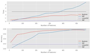
We observe the convergence in terms of the accuracy of random kernel features and Nyström methods. The computation time is also smaller up to a certain number of features.

The Github repository of this article can be found here.

Conclusion : I hope that that this article on large scale kernel methods was useful to you at some point. Don’t hesitate to drop a comment if you have any question.