
In this article, I will discuss and summarize the paper: “Leveraging side information for speaker identification with the Enron conversational telephone speech collection” by Ning Gao, Gregory Sell, Douglas W. Oard and Mark Dredze.
Background
In conversational data such as the ones that we get in criminal investigation, we collect much more information than just the speech itself. We supposely have 2 identities between 2 nodes, who might have talked previously. We can therefore leverage graph structures to enhance speaker identification.
Data
The authors use the Enron conversational telephone speech collection, a database with several thousands of emails, and 1’731 phone calls, for a total of close to 50 hours. The authors manually transcribed 57 conversations, from 41 different speakers, among which 37 sent emails recently. 28 recording were used in trainings, and 29 in test.
Approach
For each phone recording, the authors first run a speaker identification system trained only on acoustic evidence to rank each of the candidate speakers according to the probability of their being one of the speakers in a specific call. Then, they add side information (social network features, channel features and ASR to identify known name variants) and re-rank the speaker candidates.
The Detection Cost Function (DCF) is the measure chosen to first rank the different speakers:
\[DCF = C_M P_M P_T + C_{FA} P_{FA}(1 − P_T )\]Where \(C_M\) is the cost of misses, \(C_{FA}\) is the cost of false alarms (both set to 1), and the prior probability \(P_t\) is set to 0.03.
Then, to evaluate the identification, authors use the classification error which computes how often the correct speaker is given the highest score. The mean reciprocal rank (MRR) is also used as a metric on the produced rankings.
Concretely, in a call with 2 speakers, the process is:
- a list of speakers is made for speaker 1 in the call
- a list of speakers is made for speaker 2 in the call
- remove speaker 1 from list 2
- remove speaker 2 from list 1
- compute the harmonic mean of the ranks of speaker 1 and 2: \(R = \frac{n}{\sum_{i=1}^n \frac{1}{r_i}} -1\)
Where \(r_i\) is the rank of the ground truth speaker in list \(i\) and \(n\) is the number of list, e.g. 2 in a simple phone call. \(R\) now stands for the harmonic expected rank.
If all the speakers are in the right position, i.e. 1, we end up with \(R = \frac{n}{n} - 1 = 0\) which is the best score possible.
Speaker identification
First, the recording contain multiple speakers. Speaker diarization was necessary (used i-vector segments to estimate the bounding marks).
The resulting audio samples were fed into the speaker identification system using an i-vector baseline. The UBM and the total variability matrix (T) are trained on the Fisher English corpus, and the PLDA is trained on the NIST SRE 04, 05, 06 and 08.
This baseline reaches a DCF of 0.67, classification error of 0.56 and harmonic expected rank R of 0.73.
Re-ranking
Social Networks
We have past emails for most speakers in the database. Therefore, we can expect the users to be speaking much more frequently over the phone if they exchange a lot of emails. We can therefore build an edge for every email between 2 speakers (or if they were both in CC). The weight of the edge is the frequency of the communication between 2 speakers.
A score is then computed for each pair, defined as:
\[s_p = \frac{1}{2} ((1 + \frac{e_l}{\sum e}) s_l + (1 + \frac{e_r}{\sum e}) s_r)(1 + \frac{e_{lr}}{\sum e})\]Where:
- \(e_l\) is the sum of the edge weights connected to the left speaker
- \(e_r\) is the sum of the edge weights connected to the right speaker
- \(\sum e\) is the sum of all edge weights in the network
- \(\frac{e_l}{\sum e}\) is therefore high if the left speaker is a frequent communicant
- \(e_{lr}\) is the edge weight between left speaker and right speaker
- \(s_l\) is the acoustic score of left speaker
- \(s_r\) is the acoustic score of right speaker
We end-up with pairs of speakers that are the most likely to have been in this call, by leveraging some simple graph features (number of communications, i.e relative degree, and weights between A and B).
The same approach was done by leveraging how often people talk over the phone to build the network (rather than by email). My personal take would have been to use both.
Results are displayed here:
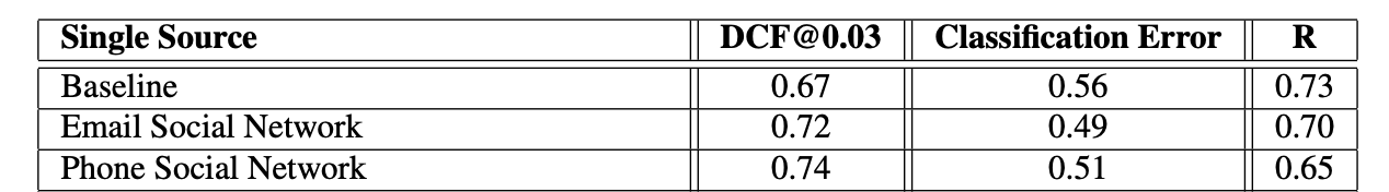
This table suggests that:
- DCF gets worse when using network information
- classification error is improved in both cases
- the harmonic expected rank is improved
Communication channel
Some speakers are often identified on some communication channels, whereas others might talk on different channels. The authors propose a new metric to weight the score by the likelihood of having speaker \(c\) talking over channel \(q\) depending on how frequently he talked on that channel \(\frac{f_i}{\sum_q f_q}\) :
\[s_c^{'} = (1 + \frac{\lambda f_i}{\sum_{q=1}^m f_q}) s_c\]Where \(\lambda\) is a simple weight factor.
Name Mention
Finally, authors extract information from the text using an ASR system and try to identify the name of the speakers. I won’t dive too much into this part, because for criminal networks, we can safely suppose that it is rarely the case.
Results
Overall results, combining several re-ranking techniques too, are presented in the table below:
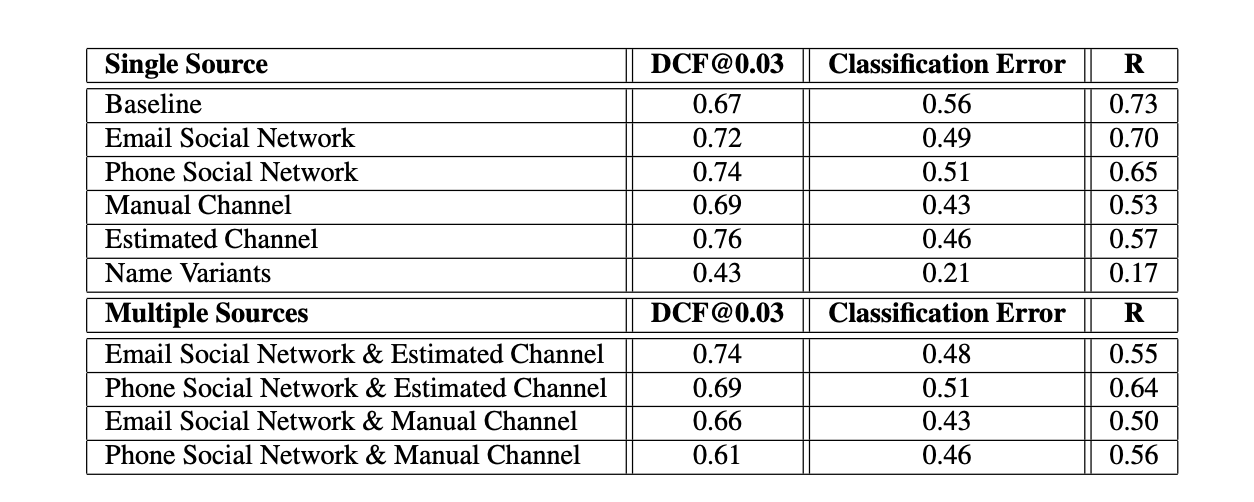
It is worth noting that:
- DCF is hardly improved by the network strcture
- Classification error is greatly improved
- the harmonic expected rank is greatly improved too
Discussion
I would have liked to see a combination of the email and phone networks, since in criminal networks, you would typically combine all sources that you have. I do also believe that there are many other ways to approach this task. However, this work, which is one of the few to address the notion of speaker identification and social networks, shows promising results.