So far, we covered the main kind of graphs, and the most basic characteristics to describe a graph. We’ll now cover into more details graph analysis/algorithms and the different ways a graph can be analyzed.

To understand the context, here are some use cases for graph algorithms :

real-time fraud detection
real-time recommendations
streamline regulatory compliance
management and monitoring of complex networks
identity and access management
social applications/features
…

3 main categories of graph algorithms are currently supported in most frameworks (networkx in Python, or Neo4J for example) :

pathfinding: identify the optimal path, evaluate route availability and quality. This can be used to identify the quickest route or traffic routing for example.
centrality: determine the importance of the nodes in the network. This can be used to identify influencers in social media for example or identify potential attack targets in a network.
community detection: evaluate how a group is clustered or partitioned. This can be used to segment customers and detect fraud for example.

For what comes next, open a Jupyter Notebook and import the following packages :

import numpy as np
import random
import networkx as nx
from IPython.display import Image
import matplotlib.pyplot as plt

If you have not already installed the networkx package, simply run :

pip install networkx

The following articles will be using the latest version 2.x of networkx. NetworkX is a Python package for the creation, manipulation, and study of the structure, dynamics, and functions of complex networks.

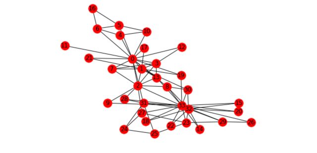
To illustrate the different concepts we’ll cover and how it applies to graphs we’ll take the Karate Club example. This graph is present in the networkx package. It represents the relations of members of a Karate Club. However, due to a disagreement of the founders of the club, the club has recently been split in two. We’ll try to illustrate this event with graphs.

First, load and plot the graph :

n=34
m = 78
G_karate = nx.karate_club_graph()

pos = nx.spring_layout(G_karate)
nx.draw(G_karate, cmap = plt.get_cmap('rainbow'), with_labels=True, pos=pos)

I. Pathfinding and Graph Search Algorithms

Pathfinding algorithms try to find the shortest path between two nodes by minimizing the number of hops.
Search Algorithms does not give the shortest path. Instead, they explore graphs considering neighbors or depths of a graph.

1. Search Algorithms

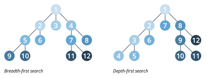
There are two main graph search algorithms :

Breadth-First Search (BFS) that explore each node’s neighbor first, then neighbors or the neighbors…
Depth-First Search (DFS) which try to go down a path as much as possible, and visit new neighbors if possible

2. Pathfinding algorithms

a. Shortest Path

Shortest Path calculates the shortest weighted (if the graph is weighted) path between a pair of nodes. It is used to identify optimal driving directions or degree of separation between two people on a social network for example.

In Python :

# Returns the shortest path between each node
nx.shortest_path(G_karate)

Returns a list of the minimal path between each node of the graph :

{0: {0: [0],
    1: [0, 1],
    2: [0, 2],
    ...

b. Single-Source Shortest Path

The Single Source Shortest Path (SSSP) computes the shortest path from a given node to all other nodes in the graph. It is often used for routing protocol for IP networks for example.

c. All Pairs Shortest Path

The All Pairs Shortest Path (APSP) algorithm computes the shortest path length between all pairs of nodes. It is quicker than calling the Single Source Shortest Path for every pair of nodes.

This algorithm can typically be used to determine traffic load expected on different segments of a transportation grid.

# Returns shortest path length between each node
list(nx.all_pairs_shortest_path_length(G_karate))

Which returns :

[(0,
    {0: 0,
    1: 1,
    2: 1,
    3: 1,
    4: 1,
    ...

d. Minimum Weight Spanning Tree

A minimum spanning tree is a subgraph of the graph (a tree) with the minimum sum of edge weights. A spanning forest is a union of the spanning trees for each connected component of the graph.

from networkx.algorithms import tree
mst = tree.minimum_spanning_edges(G_karate, algorithm='prim', data=False)
edgelist = list(mst)
sorted(edgelist)

[(0, 1),
(0, 2),
(0, 3),
(0, 4),
(0, 5),
(0, 6),
...

II. Community detection

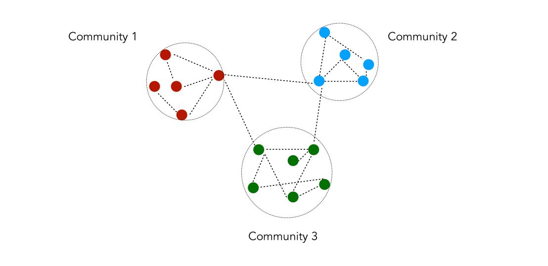
Community detection is a process by which we partition the nodes into a set of groups/clusters according to a certain quality criterion. It is typically used to identify social communities, customers behaviors or web pages topics.

A community is a set of nodes densely connected internally and/or sparsely connected externally. There is however no universal definition that one can give to define communities.

The process to identify communities is the following :

define a quality criterion
design an algorithm to optimize this criterion

We’ll try to define this into more details.

Notations

Number of nodes in the graph : \(n\)
Nodes in the community : \(S\)
Number of edges in \(S\) : \(m_s\)
Number of edges in the graph : \(m\)
Number of nodes in \(S\) : \(n_s\)
Number of edges between \(S\) and the rest of the graph : \(O_s\)

We are now ready to define quality criteria.

Quality criteria

Quality criteria might be based on :

internal connections
external connections
both

Based on internal connections :

Internal density of edges : \(\frac {m_s} {n_s \frac {(n_s-1)} {2}}\)
Average internal degree : \(\frac {2m_s} {n_s}\)

Based on external connections :

Expansion : \(\frac {O_s} {n_s}\)
Ratio Cut : \(\frac {O_s} {n_s ( n- n_s)}\)

Based on both :

Conductance : \(\frac {O_s} {2 m_s + O_s}\)
Normalized cut : \(\frac {O_s} {2m_s + O_s} + \frac {O_s} {2(m-m_s) + O_s}\)
Modularity : \(\frac {1} {4} (m_s - E(m_s))\)

A note on modularity : \(E(m_s)\) is computed with respect to a random process which preserves the degree of each node. Each degree is split into two parts. Each part is combined with another randomly.

Modularity is defined by : \(\frac {1} {2m} \sum_{i,j} (A_{ij} - \frac {d_i d_j} {2m} ) I_{C_i = C_j}\)

However, finding communities maximizing the modularity is an exponentially complex task in the number of groups. It can easily get very costly with a few hundred nodes. For this reason, methods such as the Louvain method have been developed.

We’ll now cover computationally efficient techniques that scale pretty easily :

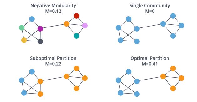
Louvain Modularity

Before defining the Louvain method, it is important to define the notion of modularity. Modularity is a measure of how well groups have been partitioned into clusters :

The pseudo-code of the Louvain method is the following :

Assign a community to each node at first
Alternate the next 2 steps until convergence :
- Optimize local modularity. For each node, create a new community with neighboring node maximizing modularity
- Create a new weighted graph. Communities of the previous step become nodes of the graph

This might seem a bit confusing right now. The only thing we’re doing is to group the closest nodes so that we optimize the modularity criteria.

Note that there is no theoretical guarantee of the Louvain method, but it works well in practice.

Strongly Connected Components

The Strongly Connected Components (SCC) algorithm finds sets of connected nodes in a directed graph where each node is reachable in both directions from any other node in the same set. It is often used early in a graph analysis process to give us an idea of how our graph is structured, for example, to explore financial statements data when we look at who owns shared in what company.

Weak Connected Components (Union Find)

The Weakly Connected Components, or Union Find algorithm finds sets of connected nodes in a directed graph where each node is reachable from any other node in the same set. It only needs a path to exist between pairs of nodes in one direction, whereas SCC needs a path to exist in both directions. As with SCC, Union Find is often used early in analysis to understand a graph’s structure.

Union Find is a pre-processing step that is essential before any kind of algorithm, to understand the graph’s structure.

We can test for connected directed graphs using :

nx.is_weakly_connected(G)
nx.is_strongly_connected(G)

Or for undirected graphs using :

nx.is_connected(G_karate)

Which returns a boolean.

Make sure to check the Networkx documentation on the Connectivity for implementations.

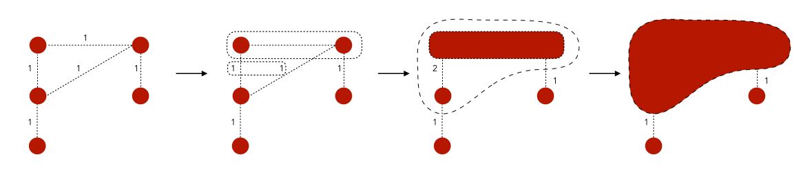
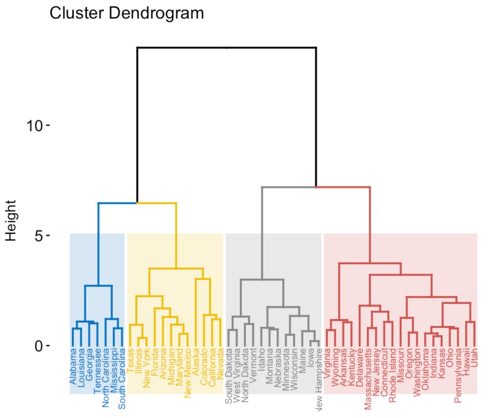
Hierarchical Clustering

In hierarchical clustering, we build a hierarchy of clusters. We represent the clusters under a form a dendrogram :

The idea is to analyze community structures at different scales. We build the dendrogram bottom-up. We start with a cluster at each node and merge the two “closest” nodes.

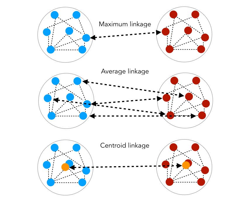
But how do we measure close clusters ? We use similarity distances. Let \(d(i,j)\) be the length of the shortest path between \(i\) and \(j\).

Maximum linkage : \(D( C_1, C_2 ) = min_{i ∈ C_1, j ∈ C_2} d(i,j)\)
Average linkage : \(D( C_1, C_2 ) = \frac {1} { \mid C_1 \mid \mid C_2 \mid } \sum_{i ∈ C_1, j ∈ C_2} d(i,j)\)
Centroïd linkage : \(D(C_1, C_2) = d(G_1, G_2)\) where \(G_1\) and \(G_2\) are the centers of \(C_1, C_2\).

The similarity distances can be illustrated as follows :

Back to our Karate example. Then, before applying hierarchical clustering, we need to define the matrix of distances between each node.

pcc_longueurs=list(nx.all_pairs_shortest_path_length(G_karate))
distances=np.zeros((n,n))

# distances[i, j] is the length of the shortest path between i and j
for i in range(n):
    for j in range(n):
        distances[i, j] = pcc_longueurs[i][1][j]

Now, we’ll use the AgglomerativeClustering function of sklearn to identify hierarchical clustering.

from sklearn.cluster import AgglomerativeClustering

clustering = AgglomerativeClustering(n_clusters=2,linkage='average',affinity='precomputed').fit_predict(distances)

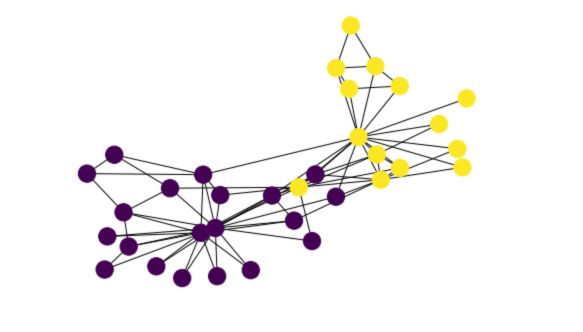
And finally, draw the resulting graph with colors depending on the cluster :

nx.draw(G_karate,  node_color = clustering)

Clustering Coefficient

The clustering coefficient measures how well two nodes tend to cluster together.

A local clustering coefficient measures how close a node \(i\) and its neighbors are to being a complete graph.

\[C_i = \frac { Triangles_i} {Triples_i}\]

The local clustering coefficient is a ratio of the number of triangles centered at node \(i\) over the number of triples centered at node \(i\).

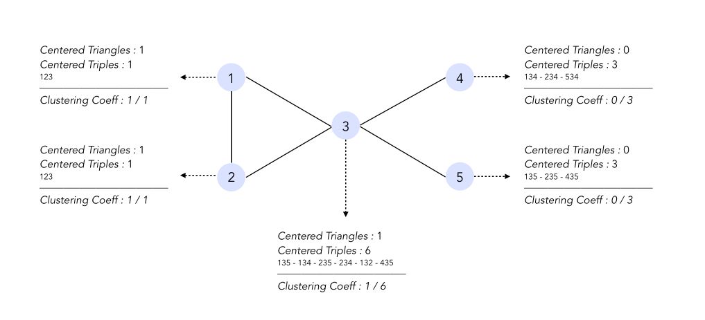
A global coefficient measures the density of triangles (local clusters) in the graph :

\[CC = \frac {1} {n} \sum_i C_i\]

In the graph shown above, the clustering coefficient is equal to :

\[CC = \frac {1} {5} ( 1 + 1 + \frac {1} {6} + 0 + 0 ) = \frac {13} {30}\]

Erdos-Rényi

For Erdos-Rényi random graphs, \(E[CC] = E[C_i] = p\) where \(p\) the probability defined in the previous article.

Barabàsi - Albert

For Baràbasi-Albert random graphs, the global clustering coefficient follows a power law depending on the number of nodes. The average clustering coefficient of nodes with degree \(k\) is \(C(k) \propto k^{-1}\).

Nodes with a low degree are connected to other nodes in their community. Nodes with high degrees are linked to nodes in different communities.

For a given graph, in networkx, the clustering coefficient can be easily computed. First, let’s begin with the local clustering coefficients :

# List of local clustering coefficients
list(nx.clustering(G_barabasi).values())

13636363636363635,
2,
07602339181286549,
04843304843304843,
09,
055384615384615386,
07017543859649122,
...

And average the results to find the global clustering coefficient of the graph :

# Global clustering coefficient
np.mean(list(nx.clustering(G_barabasi).values()))

0.0965577637155059

III. Centrality algorithms

It is hard to give a universal measure of centrality. Centrality measures express by how much a node is important when we want to identify important web pages, bottlenecks in transportation networks…

A walk is a path which can go through the same node several times. Centrality measures vary with the type of walk considered and the way of counting them.

PageRank Algorithm

PageRank estimates a current node’s importance from its linked neighbors and then again from their respective neighbors. Although popularized by Google, it’s widely recognized as a way of detecting influential nodes in any network.

It is for example used to suggest connections on social networks.

PageRank is computed by either iteratively distributing one node’s rank (originally based on the degree) over its neighbors or by randomly traversing the graph and counting the frequency of hitting each node during these walks.

Degree Centrality

Degree Centrality measures the number of incoming and outgoing relationships from a node.

\(C(X_i) = d_i\), measuring the number of walks of length 1 ending at node \(i\)

Degree Centrality is used to identify the most influential persons on a social network for example.

c_degree = nx.degree_centrality(G_karate)
c_degree = list(c_degree.values())

Eigenvector Centrality

Eigenvector Centrality represents the number of walks of infinite length ending at node \(i\). This gives more importance to nodes with well-connected neighbors.

\(C(X_i) = \frac {1} {\lambda} \sum_j A_{ij} C(X_j)\) were \(\lambda\) the largest eigenvalue of \(A\).

c_eigenvector = nx.eigenvector_centrality(G_karate)
c_eigenvector = list(c_eigenvector.values())

Closeness Centrality

Closeness Centrality is a way of detecting nodes that can spread information efficiently through a graph. It is used to research organizational networks where individuals with high closeness centrality are in a favorable position to control and acquire vital information and resources with the organization, for example, networks of fake news accounts or terrorist cells.

\(C(X_i) = \frac {1} { \sum_{j ≠ i} d(i,j) }\), is inversely proportional to the sum of lengths of the shortest paths to other nodes.

c_closeness = nx.closeness_centrality(G_karate)
c_closeness = list(c_closeness.values())

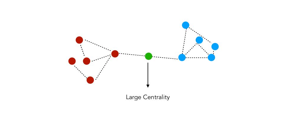
Betweenness Centrality

Betweenness Centrality is a way of detecting the amount of influence a node has over the flow of information in a graph. It is often used to find nodes that serve as a bridge from one part of a graph to another, for example in package delivery process or a telecommunication network.

\(C(X_i) = \sum_{j≠i, i≠k} \frac { \sigma_{jk}(i) } { \sigma_{jk} }\) where :

\(\sigma_{jk}\) the number of shortest paths between \(j\) and \(k\)
\(\sigma_{jk}(i)\) the number of shortest paths between \(j\) and \(k\) going through \(i\)

The betweenness centrality measures the number of times a node acts as a bridge between two nodes. For example :

c_betweenness = nx.betweenness_centrality(G_karate)
c_betweenness = list(c_betweenness.values())

In Python, the implementation relies on the built-in functions of networkx :

# Plot the centrality of the nodes
plt.figure(figsize=(18, 12))
f, axarr = plt.subplots(2, 2, num=1)
plt.sca(axarr[0,0])
nx.draw(G_karate, cmap = plt.get_cmap('inferno'), node_color = c_degree, node_size=300, pos=pos, with_labels=True)
axarr[0,0].set_title('Degree Centrality', size=16)

plt.sca(axarr[0,1])
nx.draw(G_karate, cmap = plt.get_cmap('inferno'), node_color = c_eigenvector, node_size=300, pos=pos, with_labels=True)
axarr[0,1].set_title('Eigenvalue Centrality', size=16)

plt.sca(axarr[1,0])
nx.draw(G_karate, cmap = plt.get_cmap('inferno'), node_color = c_closeness, node_size=300, pos=pos, with_labels=True)
axarr[1,0].set_title('Proximity Centrality', size=16)

plt.sca(axarr[1,1])
nx.draw(G_karate, cmap = plt.get_cmap('inferno'), node_color = c_betweenness, node_size=300, pos=pos, with_labels=True)
axarr[1,1].set_title('Betweenness Centrality', size=16)

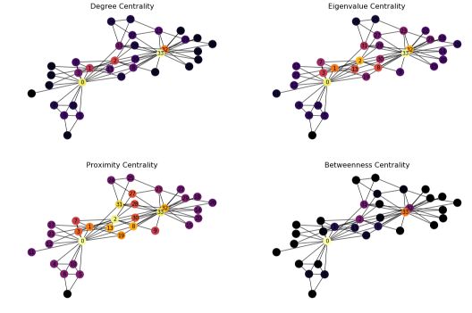
We observe that the different nodes highlighted by the centrality measures are quite distinct. Betweenness centrality, for example, produces results far from the other methods.

Conclusion : I hope that this article was helpful. Don’t hesitate to drop a comment if you have any question.

Sources :

A Comprehensive Guide to Graph Algorithms in Neo4j
Networkx Documentation

Graph Algorithms

Maël Fabien