
You might have already heard of graph analysis previously. In this article, we’ll cover the basic graph notions.
For what comes next, open a Jupyter Notebook and import the following packages :
import numpy as np
import random
import networkx as nx
from IPython.display import Image
import matplotlib.pyplot as plt
If you have not already installed the networkx package, simply run :
pip install networkx
The following articles will be using the latest version 2.x of networkx. NetworkX is a Python package for the creation, manipulation, and study of the structure, dynamics, and functions of complex networks.
What is a Graph?
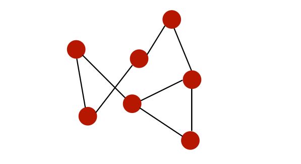
A graph is a collection of nodes that are interconnected. For example, a very simple graph could be :
Graphs can be used to represent :
- social networks
- web pages
- biological networks
- …
What can we do on a graph?
- study topology and connectivity
- community detection
- identification of central nodes
- …
In our notebook, let’s import our first pre-built graph :
# Load the graph
G_karate = nx.karate_club_graph()
# Find key-values for the graph
pos = nx.spring_layout(G_karate)
# Plot the graph
nx.draw(G_karate, cmap = plt.get_cmap('rainbow'), with_labels=True, pos=pos)
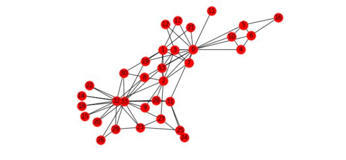
What does this graph represent? “A social network of a karate club was studied by Wayne W. Zachary for a period of three years from 1970 to 1972. The network captures 34 members of a karate club, documenting links between pairs of members who interacted outside the club. During the study, a conflict arose between the administrator “John A” and instructor “Mr. Hi” (pseudonyms), which led to the split of the club into two. Half of the members formed a new club around Mr. Hi; members from the other part found a new instructor or gave up karate. Based on collected data Zachary correctly assigned all but one member of the club to the groups they joined after the split.”
Basic graph notions
A graph \(G = (V,E)\) is made of a set of :
- nodes, also called verticles, \(V = {1,...,n}\)
-
edges \(E ⊆ V \times V\)
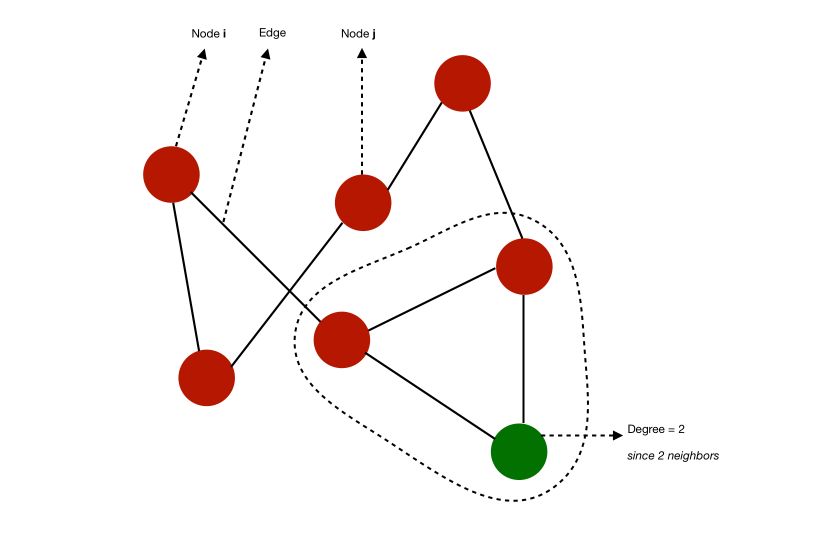
- An edge \((i,j) ∈ E\) links nodes \(i\) and \(j\). \(i\) and \(j\) are said to be neighbors.
- A degree of a node is its number of neighbors
- A graph is complete is all nodes have \(n-1\) neighbors, i.e all nodes are connected in every possible way.
- A path from \(i\) to \(j\) is a sequence of edges that goes from \(i\) to \(j\). This path has a length equal to the number of edges
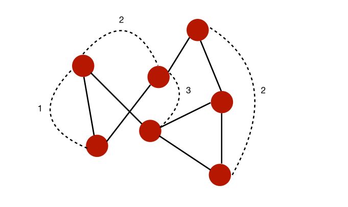
- The diameter of a graph is the length of the longest path among all the shortest path that link any two nodes
For example, in this case, we can compute some of the shortest paths to link any two nodes. The diameter would typically be 3 since the is no pair of nodes such that the shortest way to link them is longer than 3.
- The shortest path between two nodes is called the geodesic path.
- If all the nodes can be reached from each other by a given path, they form a connected component
- A graph is connected is it has a single connected component
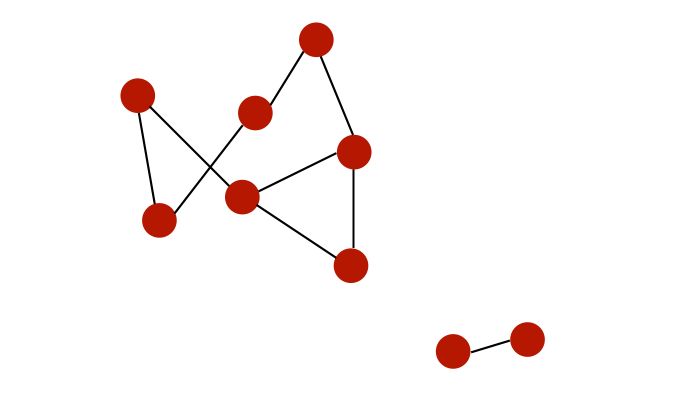
For example, here is a graph with 2 different connected components :
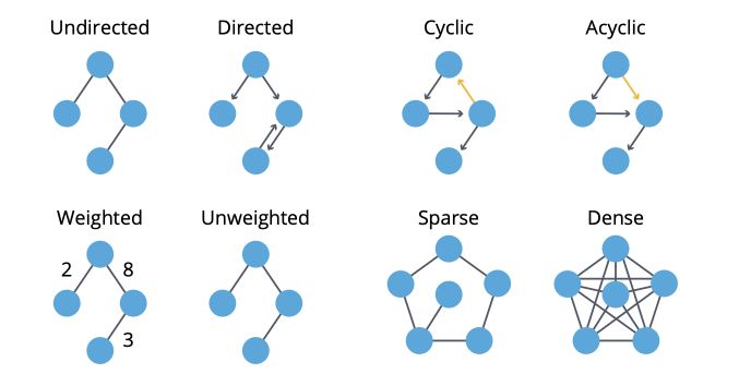
- A graph is directed if edges are ordered pairs. In this case, the “in-degree” of \(i\) is the number of incoming edges to \(i\), and the “out-degree” is the number of outgoing edges from \(i\).
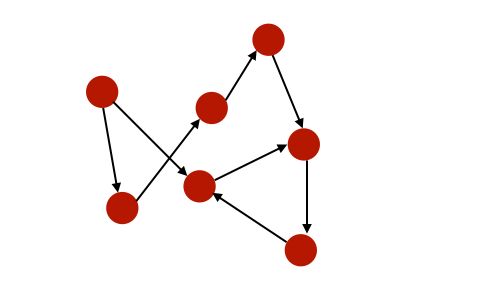
- A graph is cyclic if there are paths through relationships and nodes where you walk from and back to a particular node.
- A graph is weighted if we assign weights to either nodes or relationships.
- A graph is sparse if the number of relationships is large compared to nodes.
To summarize :
Let’s now see how to retrieve this information from a graph in Python :
n=34

G_karate.degree()
The attribute .degree() returns the list of the number of degrees (neighbors) for each node of the graph :
DegreeView({0: 16, 1: 9, 2: 10, 3: 6, 4: 3, 5: 4, 6: 4, 7: 4, 8: 5, 9: 2, 10: 3, 11: 1, 12: 2, 13: 5, 14: 2, 15: 2, 16: 2, 17: 2, 18: 2, 19: 3, 20: 2, 21: 2, 22: 2, 23: 5, 24: 3, 25: 3, 26: 2, 27: 4, 28: 3, 29: 4, 30: 4, 31: 6, 32: 12, 33: 17})
Then, isolate the values of the degrees :
# Isolate the sequence of degrees
degree_sequence = list(G_karate.degree())
Compute the number of edges, but also metrics on the degree sequence :
nb_nodes = n
nb_arr = len(G_karate.edges())

avg_degree = np.mean(np.array(degree_sequence)[:,1])
med_degree = np.median(np.array(degree_sequence)[:,1])

max_degree = max(np.array(degree_sequence)[:,1])
min_degree = np.min(np.array(degree_sequence)[:,1])
Finally, print all this information :
print("Number of nodes : " + str(nb_nodes))
print("Number of edges : " + str(nb_arr))

print("Maximum degree : " + str(max_degree))
print("Minimum degree : " + str(min_degree))

print("Average degree : " + str(avg_degree))
print("Median degree : " + str(med_degree))
This heads :
Number of nodes: 34
Number of edges: 78
Maximum degree: 17
Minimum degree: 1
Average degree: 4.588235294117647
Median degree: 3.0
On average, each person in the graph is connected to 4.6 persons.
We can also plot the histogram of the degrees :
degree_freq = np.array(nx.degree_histogram(G_karate)).astype('float')

plt.figure(figsize=(12, 8))
plt.stem(degree_freq)
plt.ylabel("Frequence")
plt.xlabel("Degre")
plt.show()
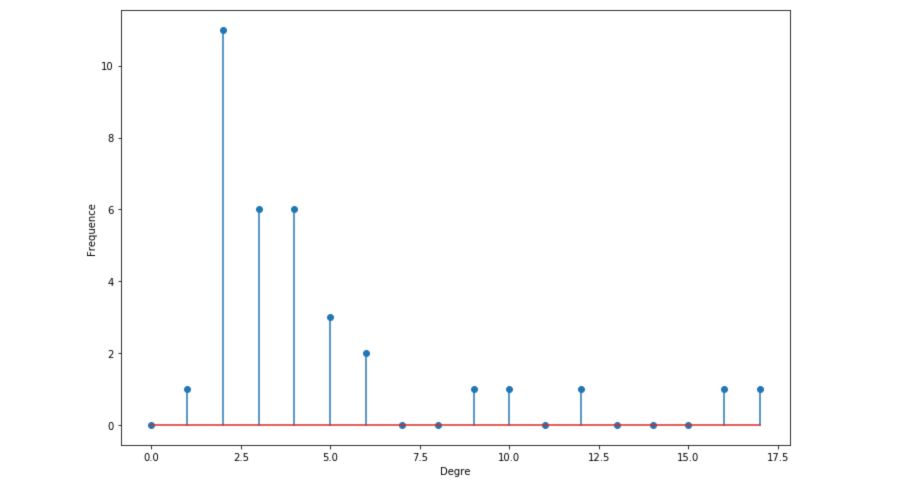
We will, later on, see that the histograms of degrees are quite important to determine the kind of graph we are looking at.
How are graphs stored?
You might now wonder how we can store complex graph structures?
There are 3 ways to store graphs, depending on the usage we want to make of it :
- at an edge list :
1   2
1   3
1   4
2   3
3   4
...
We store the ID of each pair of nodes linked by an edge.
- using the adjacency matrix, usually loaded in memory : \(A ∈ R^{n \times n}\), \(A_{i,j} = 1\) if \((i,j) ∈ E\), else 0
For each possible pair in the graph, set it to 1 if the 2 nodes are linked by an edge. \(A\) is symmetric if the graph is undirected.
- using adjacency lists :
1 : [2,3, 4]
2 : [1,3]
3:  [2, 4]
...
The best representation will depend on the usage and available memory. Graphs can usually be stored as .txt files.
Some extensions of graphs might include :
- weighted edges
- labels on nodes/edges
- feature vectors associated with nodes/edges
In the next article, we’ll explore the graph analysis basics!
Conclusion : I hope that this article introduced clearly the basis of graphs and that it does now seem clear to you. Don’t hesitate to drop a comment if you have any question.