“An anomaly is an observation that deviates so much from other observations as to arouse suspicions that it was generated by a different mechanism.”, Hawkins (1980)

Anomaly detection is used in :

network intrusions
creit card fraud detection
insurance
finance
surveillance
rental services
…

There are 3 types of anomaly detection :

supervised : we have labels for both normal data and anomalies
semi-supervised : only normal data is available, no outliers are present
unsupervised : no labels, we suppose that anomalies are rare events

The key steps in anomaly detection are the following :

learn a profile of a normal behavior, e.g. patterns, summary statistics…
use that normal profile to build a decision function
detect anomalies among new observations

Unsupervised Anomaly Detection

In unsupervised anomaly detection, we make the assumption that anomalies are rare events. The underlying data are unlabeled (no normal/abnormal label), hence the denomination. Anomalies are events supposed to be locates in the tail of the distribution.

Minimum Volume Set

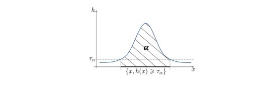
We usually estimate the region where the data is the most concentrated as the minimal region containing \(\alpha %\) of the values. This approach is called Minimum Volume Set. Samples that do not belong to the Minimum Volume Set are anomalies. For a small value of \(\alpha\) on the other hand, we tend to recover the modes.

We can define the MV Set as :

\[Q( \alpha ) = argmin_{c \in C} \{ \lambda(C), P(X \in C) ≥ \alpha \}\]

Where :

\(\alpha\) is a factor close to 1 that reflects the percentage of values in the MV Set.
\(C\) classes of measurable sets
\(\lambda\) a Lebesgue measure
\(\mu(dx)\) the unknown probability measure of the observations

The goal is to learn a minimum volume set \(Q(\alpha)\) for \(X_1, \cdots, X_n\)

There are theoretical guarantees that there exists a unique MV set at level \(\alpha\).

Let’s now make the assumption that \(\mu\) has a density \(h(X)\) that :

is bounded
has no plateau

Algorithms for anomaly detection

Plug-in technique

This technique consists in seeing MV sets as density level sets :

\[G_{\alpha}* = \{ x \in R^d : h(x) ≥ t_{\alpha} \}\]

Using a naive approach (the 2-split trick), we can :

compute a density estimator using parametric models or local averaging \(\hat{h}(x)\) based on \(X_1, \cdots, X_n\)
based on a second sample \(X_1*, \cdots, X_n*\), compute the empirical quantile corresponding to the \(\alpha\) percentile

The output is :

\[\hat{G_{\alpha}} * = \{ x: \hat{h_n(x)} ≥ \hat{h_n} ( X_{n \alpha}' ) \}\]

Unsupervised as binary classification

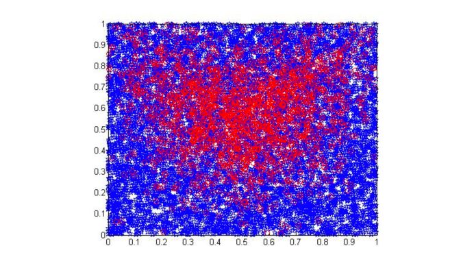
We can turn the unsupervised anomaly detection problem as a binary classification.

Suppose that our data lie into \([0,1]^d\), or that we scaled the data before. We have \(n\) points.
We then generate a new sample from the uniform distribution \(U([0,1]^d)\). We generate \(m\) points.
We assign a negative label to the generated sample.
We assign a positive label to the true sample.

We have :

\(\frac{n}{n+m} = p\) approximately.

The solution of this binary classification mimics the Bayes Classifier where we predict \(1\) on the set \(\{ x \in [0,1]^d : h(x) ≥ \frac{1-p}{p} \}\), and \(-1\) otherwise.

This solution provides a MV set at level \(\alpha = P(h(X) ≥ \frac{1}{p-1})\). We select \(\alpha\) manually, and we tune \(p\) using a grid search.

Histograms

In histograms, we suppose that we have a compact feature space, and that we build partitions \(C_1, \cdots, C_K\) formed of measurable subsets of same volume :

\[\lambda(C_1) = \cdots = \lambda(C_K)\]

The class \(G_P\) is the ensemble composed of unions of \(C_K\). We want to get the minimal number of partitions to keep in order to isolate the normal data and exclude the anomalies. More formally, we are looking for the solution of :

\[\min_{G \in P : \hat{\mu_n}(G) ≥ \alpha - \phi} \lambda(G)\]

There is a simple and fast procedure to do this :

For each class \(k = 1 \cdots K\), we compute \(\hat{\mu_n}(C_k)\), i.e the proportion of data in each class
Sort the cells by decresing order of \(\hat{\mu_n}(C_k)\)
Find the minimal value of k such that : \(\hat{k} = argmin \{ k : \sum_i \hat{\mu_n}(C_i) ≥ \alpha - \phi \}\). In other words, we exclude \(\alpha\) percent of the values based on this histogram.
The output is \(\hat{G_{\alpha}}* = U_i^{\hat{k}} C_{(i)}\)

Where \(\phi\) is a tolerance level. However, such technique is usually not flexible enough.

Decision Trees

The partition should be determined based on the data. We adopt a top-down strategy, and start from the root node \(C_{0,0}\). The volume of any cell \(C_{j,k}\) can be computed in a recursive manner.

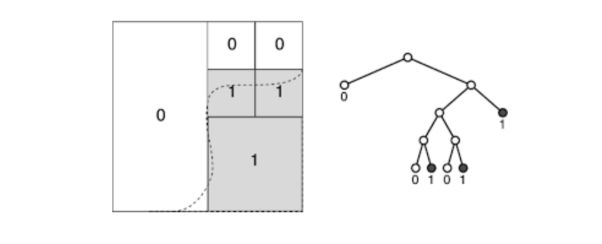
Hyperrectangless with the label 1 are subsets of the MV set estimate. At each node \(C_{j,k}\), the split leading to siblings \(C_{j+1,2k}\) and \(C_{j+1,2k+1}\) minimizes recursively the volume of the current ddecision set G under the following constraint :

\[\hat{\mu_n}(G) ≥ \alpha(-\phi)\]

To avoid overfitting, we generally prune the tree after growing it to avoid overfitting.

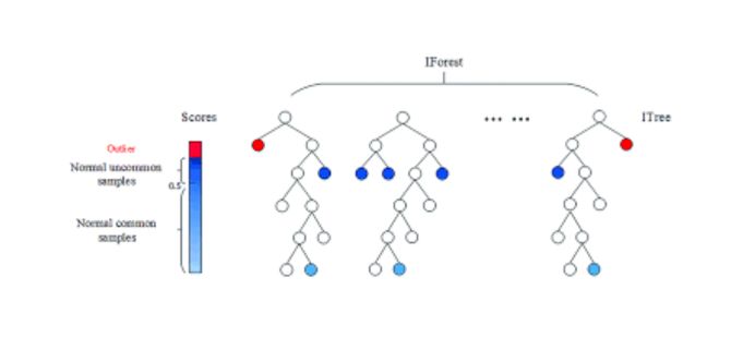
Isolation Forest

In insolation forests, we build a forest of isolation trees under the assumption that anomalies are more susceptible to isolation under random partitioning.

The main idea behind an isolation tree is to recursively (top-down) build a tree that :

chooses randomly a splitting variable
splits at value \(t\)
splits the cells if the obsevation is larger or lower than \(t\)

This process stops when a depth limit is reached usually :

Supervised Anomaly Detection

In the supervised Setup, we have pairs of data \((X,Y)\) values in \(R^d \times \{-1,+1\}\). If a data point has a positive label (Y=1), it is an anomaly. This is a classic binary classification task.

We also define a randking among anomalies, with the first data points the ones that have the highest probability to be anomalies. This is called Bipartite Ranking. It is a different approach from classification, since classification remains a local task, whereas ranking is global.

We rank and score a set of instances through a scoring function \(s(X)\) in which large number instances with label 1 appear on top of the list with high probabilities.

How do we measure the quality of a ranking?

A natural estimate of the ranking performance :

\[U(s) = P \{ (s(X) -s(X'))(Y-Y')>0\}\]

is the U-Statistic :

\[\hat{U}_n(s) = \frac{2}{n(n-1)} \sum_{1≤i<j≤n}1 \{ (s(X_i) - s(X_j))(Y_i - Y_j) > 0 \}\]

This measure is also called the rate of concording pairs, or Kendall’s association coefficient. One of the issues is that the computation of the gradients typically require to average over \(O(n^2)\) pairs.

The criterion we want to maximize is :

\[L(s) = P \{s(X^{(1)}) < \cdots < s(X^{(k)}) \mid Y^{(1)} = 1, \cdots, Y^{(k)} = K \}\]

The empirical counterpart of \(L(s)\) is really prohibitive to compute, and the maximization is even unfeasible. To overcome such issues, generalized U-Statistics using Kernels or incomplete U-Statistics using only a sample of terms can be used.

Anomaly Detection

Maël Fabien