
Boosting techniques have recently been rising in Kaggle competitions and other predictive analysis tasks. You may have heard of them under the names of XGBoost or LGBM. In this tutorial, we’ll go through Adaboost, one of the first boosting techniques discovered.
This article can also be found on Towards Data Science.
The limits of Bagging
For what comes next, consider a binary classification problem. We are either classifying an observation as 0 or as 1. This is not the purpose of the article, but for the sake of clarity, let’s recall the concept of bagging.
Bagging is a technique that stands for Bootstrap Aggregating. The essence is to select T bootstrap samples, fit a classifier on each of these samples, and train the models in parallel. Typically, in a Random Forest, decision trees are trained in parallel. The results of all classifiers are then averaged into a bagging classifier :
\[H_T(x) = 1/T \sum_t {h_t(x)}\]This process can be illustrated in the following way. Let’s consider 3 classifiers which produce a classification result and can be either right or wrong. If we plot the results of the 3 classifiers, there are regions in which the classifiers will be wrong. These regions are represented in red.
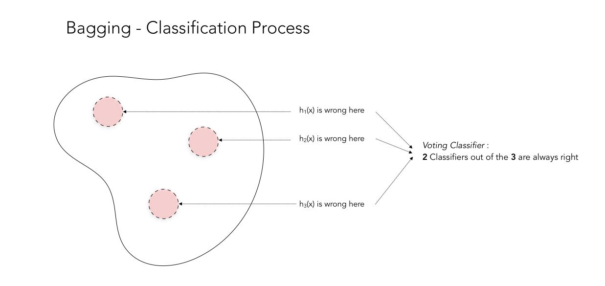
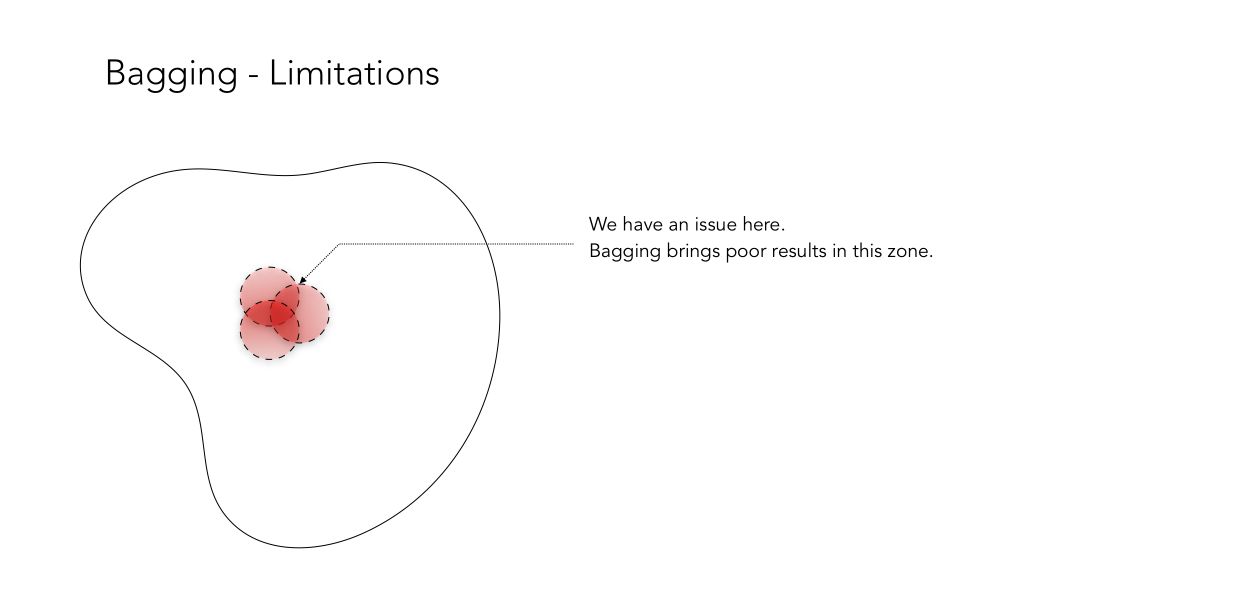
This example works perfectly since when one classifier is wrong, the two others are correct. By voting classifier, you achieve great accuracy! But as you might guess, there are also cases in which Bagging does not work properly, when all classifiers are mistaken in the same region.
For this reason, the intuition behind the discovery of Boosting was the following :
- instead of training parallel models, one needs to train models sequentially
- and each model should focus on where the previous classifier performed poorly
Introduction to Boosting
Concept
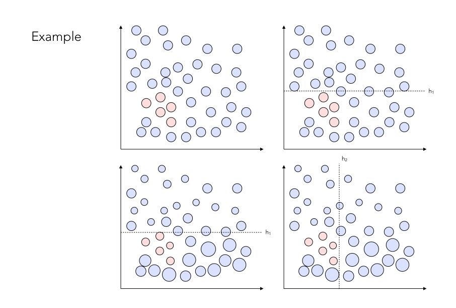
The intuition described above can be described as such :
- Train the model \(h_1\) on the whole set
- Train the model \(h_2\) with exaggerated data on the regions in which \(h_1\) performs poorly
- Train the model \(h_3\) with exaggerated data on the regions in which \(h_1\) ≠ \(h_2\)
- …
Instead of training the models in parallel, we can train them sequentially. This is the essence of Boosting!
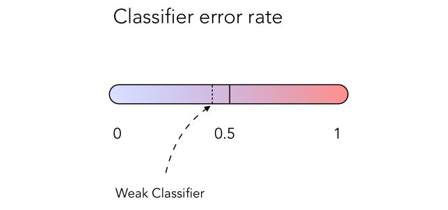
Boosting trains a series of low performing algorithms, called weak learners, by adjusting the error metric over time. Weak learners are algorithms whose error rate is slightly under 50% as illustrated below :
Weighted errors
How could we implement such classifier? By weighting errors throughout the iterations! This would give more weight to regions in which the previous classifiers performed poorly.
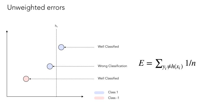
Let’s consider data points on a 2D plot. Some of them will be well classified, others won’t. Usually, the weight attributed to each error when computing the error rate is \(\frac {1} {n}\) where n is the number of data points to classify.
Now if we apply some weight to the errors :
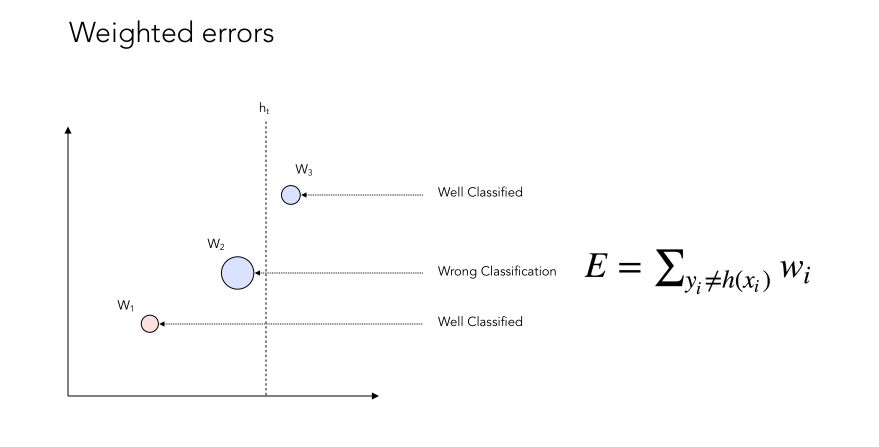
You might now notice that we give more weight to the data points that are not well classified. Here’s an illustration of the weighting process :
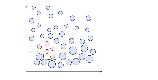
In the end, we want to build a strong classifier that may look like this :
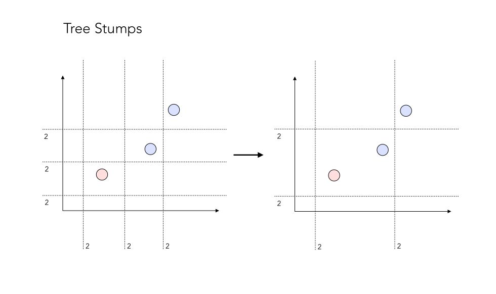
Tree stumps
One question you might ask, is how many classifiers should one implement to have it working well? And how is each classifier chosen at each step?
The answer lies in the definition of so-called tree stumps! Tree stumps defines a 1-level decision tree. The main idea is that at each step, we want to find the best stump, i.e the best data split, that minimizes the overall error. You can see a stump as a test, in which the assumption is that everything that lies on one side belongs to class 1, and everything that lies on the other side belongs to class 0.
There are a lot of combinations possible for a tree stump. Let’s see how many combinations we face in our simple example? Let’s take a minute to count them.
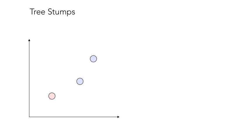
Well, the answer is… 12 ! It might seem surprising, but it’s rather easy to understand.
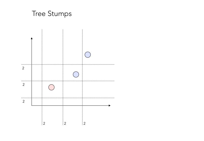
There are 12 possible “test” we could make. The “2” on the side of each separating line simply represents the fact that all points on one side could be points that belong to class 0, or class 1. Therefore, there are 2 tests embedded in it.
At each iteration \(t\), we will choose \(h_t\) the weak classifier that splits best the data, by reducing the overall error rate the most. Recall that the error rate is a modified error rate version that takes into account what has been introduced before.
Finding the best split
As stated above, the best split is found by identifying at each iteration \(t\), the best weak classifier \(h_t\), generally a decision tree with 1 node and 2 leaves (a stump). Suppose that we are trying a predict whether someone who wants to borrow money will be a good payer or not :
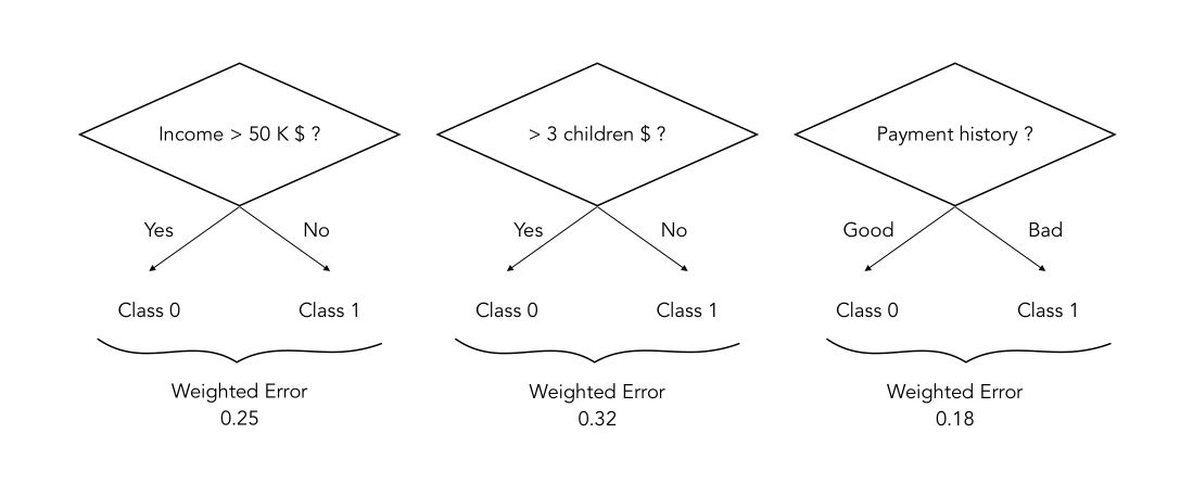
In this case, the best split at time \(t\) is to stump on the Payment history. In this case, the best split at time tt is to stump on the Payment history, since the weighted error resulting from this split is minimal.
Simply note that decision tree classifiers like these can in practice be deeper than a simple stump. This will be a hyper-parameter.
Combining classifiers
The next logical step is to combine the classifiers into a Sign classifier and depending on which side of the frontier a point will stand, it will be classified as 0 or 1. It can be achieved this way :
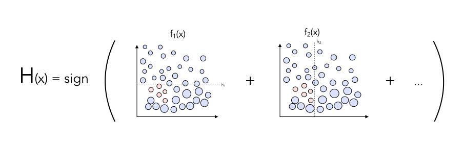
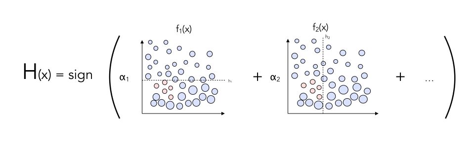
Do you see any way to potentially improve the classifier?
By adding weights \(\alpha^t\) on each classifier !
Wrapping it up
Let’s wrap up in a small pseudo-code what we covered so far.
Step 1 : Let \(w_{t}(i) = \frac {1} {N}\) where \(N\) denotes the number of training samples, and let \(T\) be the chosen number of iterations.
Step 2 : For \(t\) in \(T\) :
a. Pick \(h^t\) the weak classifier that minimizes \(\epsilon_{t}\)
\[\epsilon_{t} = \sum _{i=1}^{m} w_{t}(i)[y_{i}\neq h(x_{i})]\]b. Compute the weight of the classifier chosen :
\[\alpha_t = \frac {1} {2} ln \frac {1-\epsilon_{t}} {\epsilon_{t}}\]c. Update the weights of the training examples \(w_{t+1}^{i}\) and go back to step a).
Step 3 : \(H(x) = sign(\alpha^1 h^1(x) + \alpha^2 h^2(x) + ... + \alpha^T h^T(x))\)
If you’d like to understand the intuition behind $ w_i^{t+1} $, here’s the formula : \(w_{t+1}(i) = \frac { w_{t}(i) } { Z } e ^{- \alpha^t h^t(x) y(x)}\)
The key elements to remember from it are :
- \(Z\) is a constant whose role is to normalize the weights so that they add up to 1!
- \(\alpha^t\) is a weight that we apply to each classifier
And we’re done! This algorithm is called AdaBoost. This is the most important algorithm one needs to understand to fully understand all boosting methods.
Computation
Boosting algorithms are rather fast to train, which is great. But how come they’re fast to train since we consider every stump possible and compute exponentials recursively?
Well, here’s where the magic happens. If we choose properly \(\alpha^t\) and \(Z\), the weights that are supposed to change at each step simplify to :
\(\sum_{positive} = \frac {1} {2}\) and \(\sum_{negative} = \frac {1} {2}\)
This is a very strong result, and it does not contradict the statement according to which the weights should vary with the iterations, since the number of training samples that are badly classified drops, and their total weights is still 0.5!
- No \(Z\) to compute
- No \(\alpha\)
- No exponential
And there’s another trick: any classifier that tries to split 2 well-classified data points will never be optimal. There’s no need to even compute it.
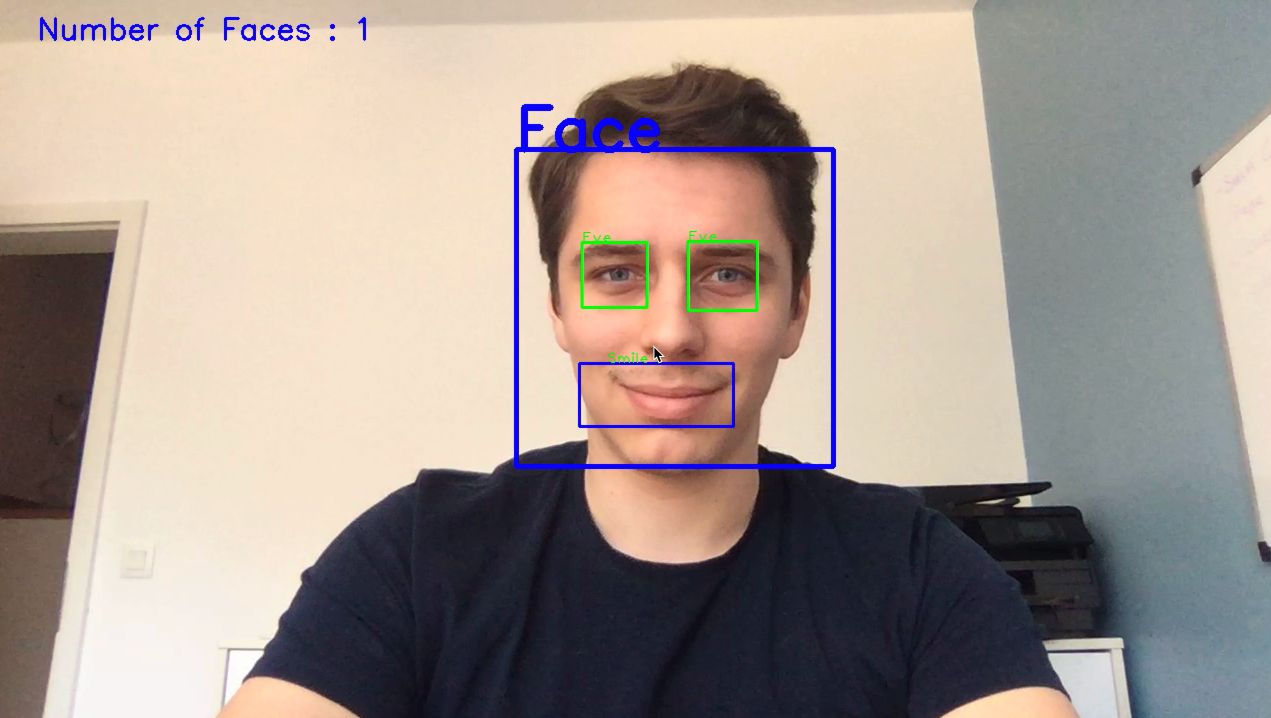
AdaBoost has for a long time been considered as one of the few algorithms that do not overfit. But lately, it has been proven to overfit at some point, and one should be aware of it. AdaBoost is vastly used in face detection to assess whether there is a face in the video or not. AdaBoost can also be used as a regression algorithm.
Let’s code!
Now, we’ll take a quick look at how to use Adaboost in Python using a simple example on a handwritten digit recognition.
import pandas as pd
import numpy as np
import matplotlib.pyplot as plt

from sklearn.ensemble import AdaBoostClassifier
from sklearn.tree import DecisionTreeClassifier

from sklearn.metrics import accuracy_score
from sklearn.model_selection import cross_val_score
from sklearn.model_selection import cross_val_predict
from sklearn.model_selection import train_test_split
from sklearn.model_selection import learning_curve

from sklearn.datasets import load_digits
Let’s load the data :
dataset = load_digits()
X = dataset['data']
y = dataset['target']
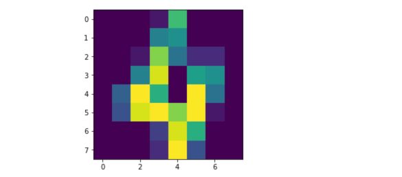
$ X $ contains arrays of length 64 which are simply flattened 8x8 images. This dataset aims to recognize handwritten digits. Let’s take a look at a given handwritten digit :
plt.imshow(X[4].reshape(8,8))
If we stick to a Decision Tree Classifier of depth 1 (a stump), here’s how to implement AdaBoost classifier :
reg_ada = AdaBoostClassifier(DecisionTreeClassifier(max_depth=1))
scores_ada = cross_val_score(reg_ada, X, y, cv=6)
scores_ada.mean()
And it should head a result of around 26%, which can largely be improved. One of the key parameters is the depth of the sequential decision tree classifiers. How does accuracy improve with depth of the decision trees?
score = []
for depth in [1,2,10] :
    reg_ada = AdaBoostClassifier(DecisionTreeClassifier(max_depth=depth))
    scores_ada = cross_val_score(reg_ada, X, y, cv=6)
    score.append(scores_ada.mean())
And the maximal score is reached for a depth of 10 in this simple example, with an accuracy of 95.8%.
The Github repository of this article can be found here.
Conclusion : I hope that this article introduced clearly the concept of AdaBoost and that it does now seem clear to you. Don’t hesitate to drop a comment if you have any question.
References :