
Sound features can be used to detect speakers, detect the gender, the age, diseases and much more through the voice.
To extract features, we must break down the audio file into windows, often between 20 and 100 milliseconds. We then extract these features per window and can run a classification algorithm for example on each window.
Start by importing the series:
x, sr = librosa.load('test.wav')
1. Statistical Features
A first easy step is to compute the mean, standard deviation, minimum, maximum, median and quartiles of the frequencies of each signal. This can be done using Numpy and it always brings value to our feature extraction. This kind of approach can be used in gender recognition for example, as seen on Kaggle.
freqs = np.fft.fftfreq(x.size)

def describe_freq(freqs):
    mean = np.mean(freqs)
    std = np.std(freqs)
    maxv = np.amax(freqs)
    minv = np.amin(freqs)
    median = np.median(freqs)
    skew = scipy.stats.skew(freqs)
    kurt = scipy.stats.kurtosis(freqs)
    q1 = np.quantile(freqs, 0.25)
    q3 = np.quantile(freqs, 0.75)
    mode = scipy.stats.mode(freqs)[0][0]
    iqr = scipy.stats.iqr(freqs)

    return [mean, std, maxv, minv, median, skew, kurt, q1, q3, mode, iqr]
This can be applied per time window or to the whole signal depending on its length.
2. Energy
The energy of a signal is the total magnitude of the signal, i.e. how loud the signal is. It is defined as:
\[E(x) = \sum_n {\mid x(n) \mid}^2\]You can compute it this way:
def rmse(x):
    return np.sum(x**2)
We can then apply this function to each time frame when building our feature extraction sliding window.
3. Root Mean Square Energy
The RMS Energy (RMSE) is simply the square root of the mean squared amplitude over a time window. It is defined by:
\[RMSE(x) = \sqrt{ \frac{1}{N} \sum_n {\mid x(n) \mid}^2}\]def rmse(x):
return np.sqrt(np.mean(x**2))
It can also be extracted with Librosa library:
import librosa

rmse = librosa.feature.rmse(x)[0]
4. Zero-Crossing Rate
The zero crossing rate indicates the number of times that a signal crosses the horizontal axis, i.e. the number of times that the amplitude reaches 0.
This can be computed using Librosa:
zero_crossings = sum(librosa.zero_crossings(x, pad=False))
This will return the total number of times the amplitude crosses the horizontal axis.
5. Tempo
An estimate of the tempo in Beats Per Minute (BPM).
tempo = librosa.beat.tempo(x)[0]
6. Mel Frequency Cepstral Coefficients (MFCC)
My understanding of MFCC highly relies on this excellent article. The MFCC are state-of-the-art features for speaker identification, disease detection, speech recognition, and by far the most used among all features present in this article.
Start by taking a short window frame (20 to 40 ms) in which we can assume that the audio signal is stationary. We then select a frame step (e.g. rolling window) of around 10 ms.
We then compute the power spectrum of each frame through a periodogram, which is inspired by the human cochlea (an organ in the ear) which vibrates at different spots depending on the frequency of the incoming sounds. To do so, start by taking the Discrete Fourrier Transform of the frame:
\[S_i(k) = \sum_{n=1}^N s_i(n)h(n) e^{-j 2 \pi k n / N}\]where:
- \(s_i(n)\) is the framed time signal (i frames)
- \(N\) is the number of samples in a Hamming Window
- \(h(n)\) is the Hamming Window
- \(K\) is the length of the DFT
To compute the periodogram estimate of the power spectrum, we apply:
\[P_i(k) = \frac{1}{N} {\mid S_i(k) \mid}^2\]Since the cochlea is not so good to discriminate between two closely spaced frequencies, especially when they are high, we take clumps of periodogram bins and sum them up. This is done by applying Mel filterbank, filters which tell us exactly how to space our filterbanks and how wide to make them. These filters are typically narrower around 0Hz and wider for higher frequencies.
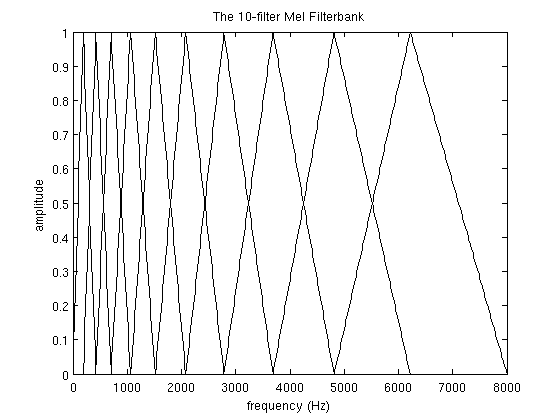
The formula to move from frequencies to Mel scale is the following:
\[M(f) = 1125 ln (1 + \frac{f}{700})\]The Mel filterbank is a set of 26 triangular filters which we apply to the periodogram power spectral estimate. Each filter is mostly made of 0’s but has a non-zero triangle in some region. We multiply the values of the periodogram by the ones of the filters.
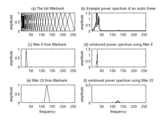
We then take the logarithm of the all those 26 series of energy of those filterbanks since we do not percieve loudness linearly, but close to logarithmically.
We finally apply a Discrete Cosine Transform to the 26 log filterbank energies in order to decorrelate the overlapping filterbanks energies. This gives us 26 coefficients, called the MFCC. Not all of them are useful, and for Automatic Speech Recognition, we typically only use the 12-13 lower values.
MFCCs are widely used to classify phonemes. They can easily be extracted using librosa library:
import librosa
x, sr = librosa.load(filename)
mfcc=librosa.feature.mfcc(x)
It returns a numpy array of size 20 (MFCC extracted) * the number of windows (for the file test.wav, 431).
array([[  22.456623 ,  -19.06088  , -164.62514  , ..., -240.06525  ,
        -257.81137  , -260.06912  ],
       [  95.18431  ,   89.34006  ,   37.92323  , ...,  171.81778  ,
         160.94362  ,   97.23265  ],
...
Since these series can get quite long as one new data point is created every 20ms, one can always extract the mean, variance, quartiles, min, max and median as a descriptive statistic at the end of an audio sample, and compare several audio samples on this basis.
7. Mel Frequency Cepstral Differential Coefficients
MFCC lacks information on the evolution of the coefficients between frames. What we can therefore do is to compute the 12 trajectories of the MFC coefficients and append them to the 12 original coefficients. This highly improves results on ASR tasks.
\[d_t = \frac{\sum_{n=1}^N n (c_{t+n} - c_{t-n})}{2 \sum_{n=1}^N n^2}\]Where:
- \(d_t\) is the delta coefficient
- \(t\) is the frame considered
- \(c_t\) is the coefficient at time \(t\) (we commonly use N=2)
8. Polyfeatures
The polyfeatures returns the coefficients of fitting an nth-order polynomial to the columns of a spectrogram. This can be easily extracted using Librosa.
poly_features=librosa.feature.poly_features(x) #order 1 by default


plt.figure(figsize=(12,8))
plt.plot(poly_features[0], label="0")
plt.plot(poly_features[1], label="1")
plt.legend()
plt.show()
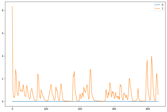
One can then apply a mean of the coefficients or get statistics to describe the series, otherwise it tends to be too much values given.
9. Tempogram
The tempo, measured in Beats Per Minute (BPM) measures the rate of the musical beat. The tempogram is a feature matrix which indicates the prevalence of certain tempi at each moment in time. Librosa has a built-in function to extract this information. It is common to focus only on the first N rows (e.g 13) of the matrix.
hop_length = 512
oenv = librosa.onset.onset_strength(y=x, sr=sr, hop_length=hop_length)
tempogram = librosa.feature.tempogram(onset_envelope=oenv, sr=sr, hop_length=hop_length)

plt.figure(figsize=(12,8))
for i in range(1,14):
    plt.plot(tempogram[i], label=i)
plt.legend()
plt.title("Tempogram")
plt.show()
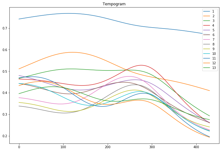
As before, one can take descriptive statistics on the output series.
10. Spectal Features
Spectral features are extracted from the spectrogram. Spectrograms offer a powerful representation of the data. It plots over the time, for a given range of frequencies, the power (dB) of a signal. This allows us to spot periodic patterns over time, and regions of activity.
The most common feature to extract is the spectral centroid. Each frame of a magnitude spectrogram is normalized and treated as a distribution over frequency bins, from which the mean (centroid) is extracted per frame.
spec_centroid = librosa.feature.spectral_centroid(x)[0]
There are other features that contain information:
spectral_bandwidth=librosa.feature.spectral_bandwidth(x)[0]
spectral_contrast=librosa.feature.spectral_contrast(x)[0]
spectral_flatness=librosa.feature.spectral_flatness(x)[0]
spectral_rolloff=librosa.feature.spectral_rolloff(x)[0]
11. Fundamental Frequency
One can also extract fundamental frequencies of a voice, which are the lowest frequencies of a periodic voice waveform. This is really useful for classifying gender, since males have lower fundamental frequencies than females in most cases. The voiced speech of a typical adult male will have a fundamental frequency from 85 to 180 Hz, and that of a typical adult female from 165 to 255 Hz.
It corresponds to the smallest value of \(T\) such that:
\[x(t)=x(t+T){\text{ for all }}t\in {\mathbb {R}}\]And the fundamental frequency is defined by:
\[f_0 = \frac{1}{T}\]12. Jitter Feature
Jitter Feature measures the deviation of periodicity in a periodic signal. It can be computed as:
\[Jitter(T) = \frac{1}{N-1} \sum_{i=1}^{N-1} \mid T_i - T_{i+1} \mid\]13. Meta features
In order to add some more features, on can create meta features. These features are the result of a regression or a classification algorithm that is ran halfway through the feature extraction process. We can for example train an algorithm to detect gender based on MFCC features, and for each new sample, predict whether this is a male or a female and add it as a features.
Among meta features, the most popular are:
- gender
- age category
- ethnicity / accent
- diseases
- emotions
- audio quality
- fatigue level
- stress level
14. Dimension reduction
One common issue when dealing with audio features is the number of features created. It can easily exceed 1’000 features on a set of audio samples, and we therefore need to think of dimension reduction techniques.
The most common unsupervised approaches are:
- Principal Component Analysis (PCA)
- K-means clustering
And for supervised approaches:
- Supervised Dictionary Learning (SDL)
- Linear Discriminant Analysis
- Variational Autoencoders
Most techniques are easy to implement using scikit-learn, but since it’s a bit less common, here’s how to implement the SDL approach:
# supervised dictionary learning
from sklearn.decomposition import MiniBatchDictionaryLearning
dico_X = MiniBatchDictionaryLearning(n_components=50, alpha=1, n_iter=500).fit_transform(X)
dico_Y = MiniBatchDictionaryLearning(n_components=50, alpha=1, n_iter=500).fit_transform(Y)
Conclusion: I hope you enjoyed this article. If you think about other features, please let me know in the comments !