Introduction to Continuous Signal Processing

I am relying on the excellent series on Youtube by Iman: Signal Processing 101 for this series of articles.

Note: This series focuses on continuous signal processing. I am also working on a digital/discrete signal processing series.

1. What is signal processing?

A signal is a time-varying physical process.

Signals can be :

• voice
• videos or images
• temperature records
• stock prices
• health records
• …

The act of processing a signal using a system is called signal processing. A signal contains information. A system processes this information.

Signal processing is implied when you:

• make a phone call
• use a voice assistance
• listen to the radio
• edit a picture
• …

2. Signal representation

Signal can be :

• 1-dimensional : On a voice record for example, each point can be represented on a value vs. time plot. If you know the time, you can retrieve the value.
• 2-dimensional: An image is 2 dimensional, since you need both x and y to characterize the value of a pixel on an image
• 3-dimensional: A video is made of a sequence of images. You need x, y and the index of the image t to know the value of a pixel.

This is called signal representation. We will however focus on 1-dimensional signals.

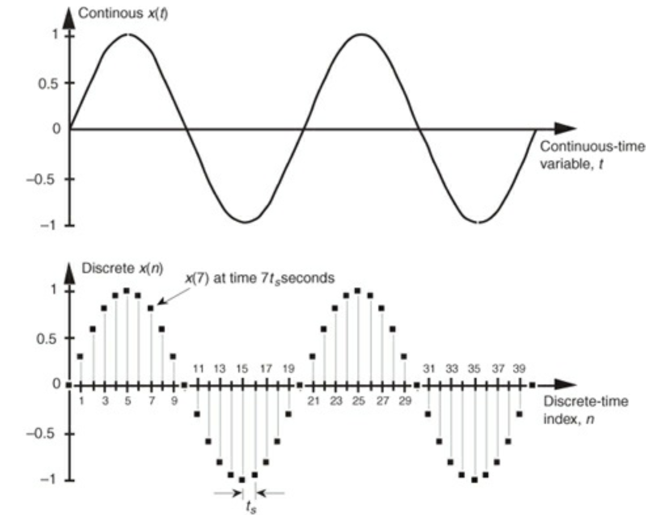
3. Discrete vs. Continuous

Signal processing is divided in 2 categories:

• continuous/analog signal processing : a signal continuous in time taking continuous range of amplitude values, defined for all times.
• discrete/digital signal processing : a discrete signal for which we only know values of the signal at discrete points in time.

A 1-dimensional continous signal could for example be:

\[x(t) = sin(2 \pi f_o t)\]

Where:

• t represents the time
• \(f_o\) represents the frequency, in Hz (number of cycles per second)
• \(2 \pi f_o t\) is an angle measured in radians

A discrete-time signal quantizes the time and the signal amplitude. We might have a discrete signal taking the following form:

(0, 0)
(1, 0.31)
(2, 0.59)
(3, 0.81)
...

Where the first value is the index, and the second is the value. The discrete signal can be represented as :

\[x(n) = sin(2 \pi f_o n t_s)\]

Where:

• n is the index (0, 1, 2, 3…)
• \(t_s\) is the time sample, i.e. the time between 2 indexs

Continuous and discrete signals can be represented as such:

4. Signal transformation

4.a. Continuous

We can apply transformations to a continuous signal \(x(t)\). For example:

• \(x(2t)\) : doubles the speed of a signal. We talk about signal compressing in time direction.
• \(x(t/2)\) : reduces by 2 the speed of a signal. We talk about signal expansion in time direction.
• \(x(-t)\) : time reversal transformation.
• \(x(t+2)\) : time shifting transformation to the left. We play the signal two units sooner.
• \(x(t-2)\) : time shifting transformation to the right. We play the signal two units later.

Transformations applied in the parenthesis usually affect the time direction. However, transformations applied outside the parenthesis affect the value axis:

• \(2x(t)\) : magnify the amplitude. We multiply the amplitude by two. If the value of 2 is smaller than 1, we say that we compress the signal in value direction.
• \(x(t) + 2\) : shift the whole signal up by 1 unit.

To summarize, we can apply the following transformations:

• time shifting
• time scaling
• amplitude shifting
• amplitude scaling

4.b. Discrete

A Discrete System is any software operating on a discrete-time signal sequence, and producing a discrete output sequence using a transformation. A simple Discrete System can be defined by a difference equation:

\[y(n) = 2 x(n) - 1\]

The same concepts as for continuous signals regarding the transformations apply.

For what comes next, we will focus exclusively on continuous signals.

5. Signal properties

Even signals

If \(x(t) = x(-t)\) this means that the signal is symmetric around the x-axis.

We talk about even signals.

Odd signals

If \(x(t) = -x(-t)\), we reflect the signal with respect to the origin and the signal is odd.

To test if a function is even or odd or neither, just replace t by -t in the expression and check for the equality.

Periodic

A signal is periodic if the same pattern repeats for ever.

Some common periodic functions are:

• \[sin(a t)\]
• \[cos(a t)\]
• \[e^{j a t}\]

The fundamental period for these signals is \(\tau = \frac{2 \pi}{a}\).