Voice activity detection is a field which consists in identifying whether someone is speaking or not at a given moment. It can be useful to launch a vocal assistant or detect emergency situations.

In this article, we will cover the main concepts behind classical approaches to voice activity detection, and implement them in Python is a small web application using Streamlit. This article is inspired by the following repository.

High-level overview

It can be useful at first to give a high level overview of the classical approaches to Voice Activity Detection:

Read the input file and convert is to mono
Move a window of 20ms along the audio data
Calculate for each window the ratio between energy of speech band and total energy for window
If ratio is higher than a pre-defined threshold (e.g 60%), label windows as speech
Apply median filter with length of 0.5s to smooth detected speech regions
Represent speech regions as intervals of time

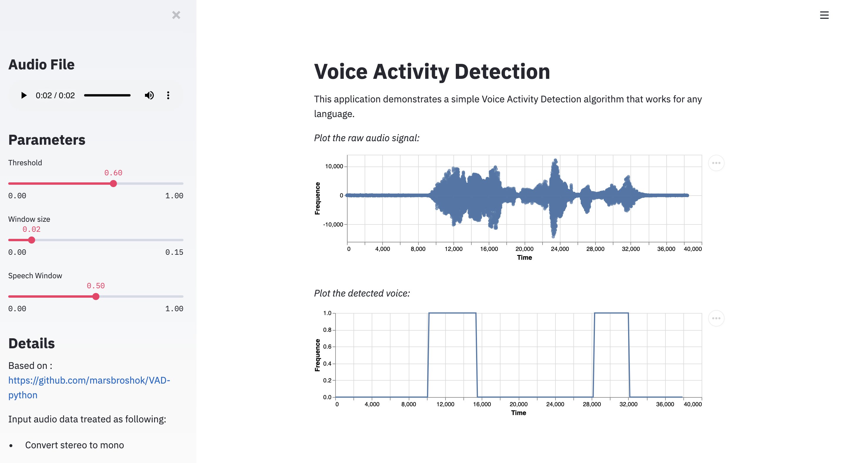
The application we will build is the following:

Read the input file and convert it to mono

In this exercise, we will only consider the case of mono signals and not stereo, meaning that we must have a single series of values, not 2. We read the files using Scipy’s wavfile module, and convert it to mono if there are 2 lists of values returned (stereo) by applying a mean of both series.

import scipy.io.wavfile as wf

filename = 'test.wav'

def _read_wav(wave_file):
	# Read the input
	rate, data = wf.read(wave_file)
	channels = len(data.shape)
	filename = wave_file

	# Convert to mono
	if channels == 2 :
		data = np.mean(data, axis=1, dtype=data.dtype)
		channels = 1
	return data

read_file = _read_wav(filename)

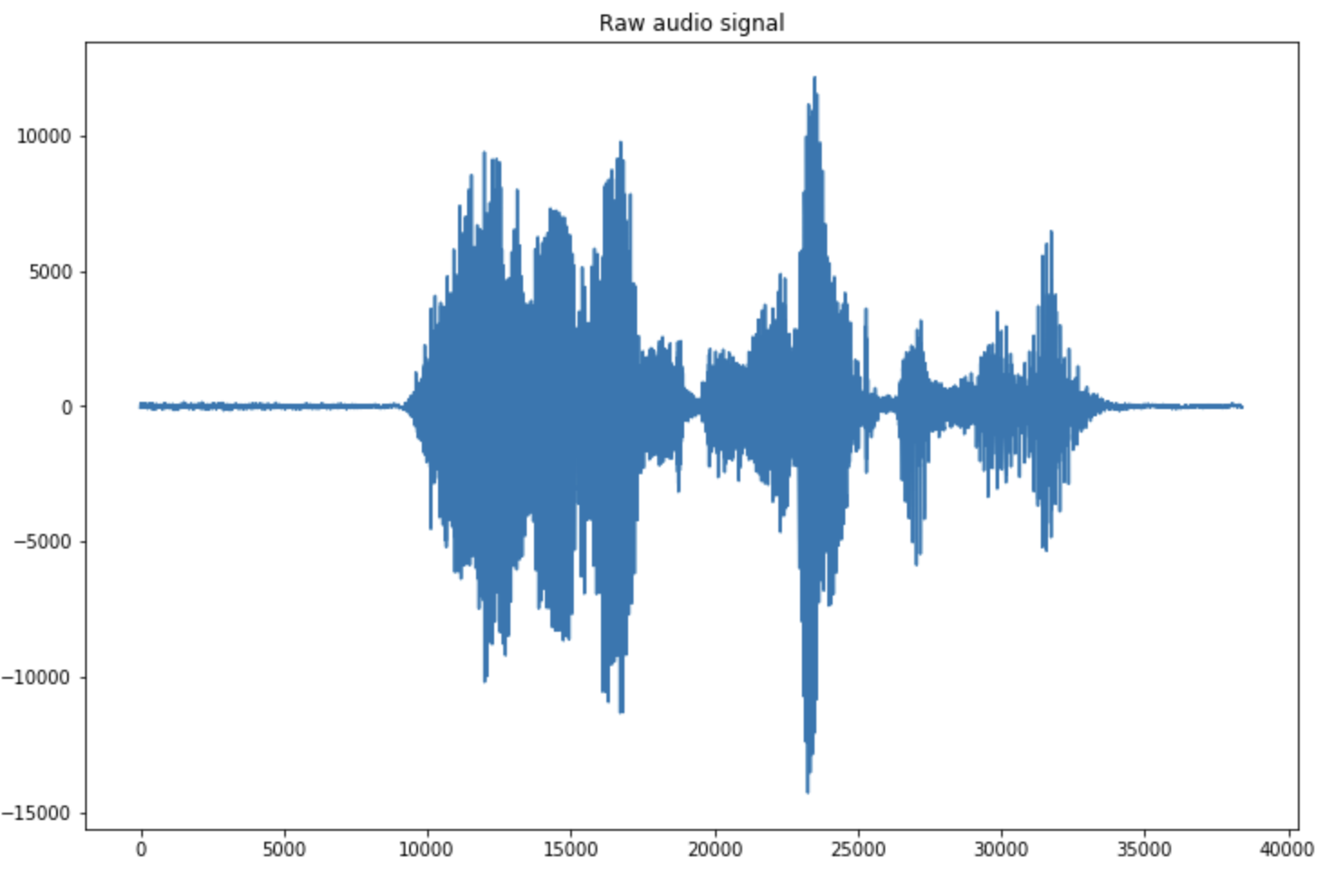
You can plot the signal in order to see which regions should be detected. In my case, the sample file contains 2 to 3 speech regions.

plt.figure(figsize=(12,8))
plt.plot(np.arange(len(data)), data)
plt.title("Raw audio signal")
plt.show()

You can already notice that there is a notion a threshold that appears. From what moment do we assume that someone is speaking? How do we split 2 regions? We’ll answer those questions as we dive deeper into the solution.

Rolling Window

The solution will take the form of a rolling window on the input data. We will determine the energy in the frequency range that usually is associated to speech, and the energy of the whole band. If the ratio is larger than a threshold, we can assume that someone is speaking.

We first need to define some constants that we will use:

SAMPLE_START = 0
SPEECH_START_BAND = 300
SPEECH_END_BAND = 3000
SAMPLE_WINDOW = 0.02
SAMPLE_OVERLAP = 0.01
THRESHOLD = 0.6

Here’s what the constants are used for:

SAMPLE_START : the start index,
SPEECH_START_BAND : the minimum frequency of a human voice
SPEECH_END_BAND : the maximum frequency of a human voice
SAMPLE_WINDOW : a 20 ms window size on which we run the algorithm
SAMPLE_OVERLAP : the amount by which we shift the window size at each step
THRESHOLD : the threshold for the energy ratio under which a sound is not tagged as a voice

The rolling window will have the following format:

while (SAMPLE_START < (len(data) - SAMPLE_WINDOW)):
    
    # Select only the region of the data in the window
    SAMPLE_END = SAMPLE_START + SAMPLE_WINDOW
    if SAMPLE_END >= len(data): 
        SAMPLE_END = len(data)-1

    data_window = data[SAMPLE_START:SAMPLE_END]
    
    # Detect speech here
    
    # Increment 
    SAMPLE_START += SAMPLE_OVERLAP

Speech Ratio

Within this data window, we now need to determine the speech ratio:

\[speech_{ratio} = \frac{\sum energy_{voice}}{\sum energy_{full}}\]

To determine the voice energy, we will only consider frequencies between 300 and 3’000 Hz, as they correspond to human voice frequencies.

The first thing we need to do is to compute the range of possible frequencies at the defined rate and given the audio sequence:

def _calculate_frequencies(audio_data):
    data_freq = np.fft.fftfreq(len(audio_data),1.0/rate)
    data_freq = data_freq[1:]
    return data_freq

This will return regular values between -8’000 and 8’000. The energy transported by a wave is directly proportional to the square of the amplitude of the wave, which can be computed using a Fast Fourrier Transform.

def _calculate_energy(audio_data):
    data_ampl = np.abs(np.fft.fft(audio_data))
    data_ampl = data_ampl[1:]
    return data_ampl ** 2

We then connect the energy with the frequency by creating a dictionary whose keys are the absolute value of the frequency, and values are the corresponding energy at that frequency.

def _connect_energy_with_frequencies(data):
    
    data_freq = _calculate_frequencies(data)
    data_energy = _calculate_energy(data)
    
    energy_freq = {}
    for (i, freq) in enumerate(data_freq):
        if abs(freq) not in energy_freq:
            energy_freq[abs(freq)] = data_energy[i] * 2
    return energy_freq

energy_freq = _connect_energy_with_frequencies(data)
sum_full_energy = sum(energy_freq.values())

The variable energy_freq should return :

{0.4166666666666667: 388888371.0778143,
8333333333333334: 378650788.74457765,
25: 139749533.30109847,
6666666666666667: 703141467.1534827,
0833333333333335: 2622893493.5843244,
5: 2214362080.232078,
 ...

As stated above, we suppose that a human voice will be anywhere between 300 and 3’000 Hz. Therefore, we sum the energy corresponding such frequencies in the time window, and we can compare it with the full sum of energies.

def _sum_energy_in_band(energy_frequencies):
    sum_energy = 0
    for f in energy_frequencies.keys():
        if SPEECH_START_BAND < f < SPEECH_END_BAND:
            sum_energy += energy_frequencies[f]
    return sum_energy

sum_voice_energy = _sum_energy_in_band(energy_freq)

Finally, we can define the speech ratio as being the quotien between the sum of the speech energy in the time window and the sum of the total energy.

speech_ratio = sum_voice_energy/sum_full_energy
speech_ratio

In this sample, it gave me : 0.68923.

Combining the loop and the speech ratio

So far, we estimated the speech ratio on the whole audio file, without using a rolling window. It is now time to combine both approaches. We will store in speech_ratio_list a list of all the speech ratios in the loop.

speech_ratio_list = []
detected_voice = []
mean_data = []

SAMPLE_START = 0

while (SAMPLE_START < (len(data) - SAMPLE_WINDOW)):
    
    # Select only the region of the data in the window
    SAMPLE_END = SAMPLE_START + SAMPLE_WINDOW
    if SAMPLE_END >= len(data): 
        SAMPLE_END = len(data)-1

    data_window = data[SAMPLE_START:SAMPLE_END]
    mean_data.append(np.mean(data_window))

    # Full energy
    energy_freq = _connect_energy_with_frequencies(data_window)
    sum_full_energy = sum(energy_freq.values())
    
    # Voice energy
    sum_voice_energy = _sum_energy_in_band(energy_freq)
    
    # Speech ratio
    speech_ratio = sum_voice_energy/sum_full_energy
    speech_ratio_list.append(speech_ratio)
    detected_voice.append(speech_ratio > THRESHOLD)
    
    # Increment 
    SAMPLE_START += SAMPLE_OVERLAP

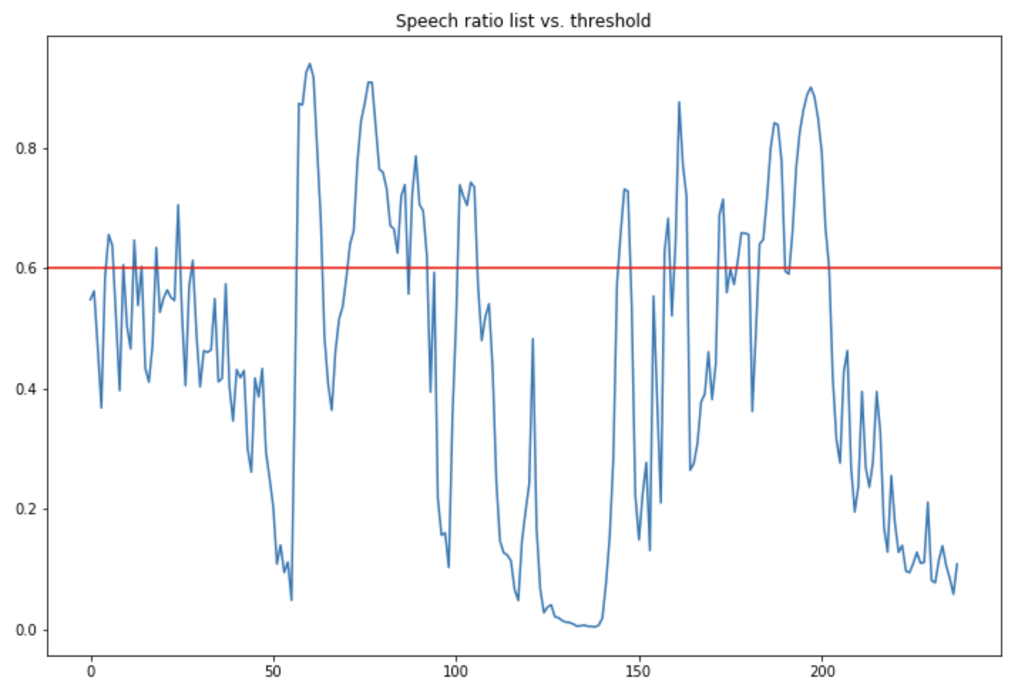
We can now compare the speech ratio list with the threshold over time:

plt.figure(figsize=(12,8))
plt.plot(speech_ratio_list)
plt.axhline(THRESHOLD, c='r')
plt.title("Speech ratio list vs. threshold")
plt.show()

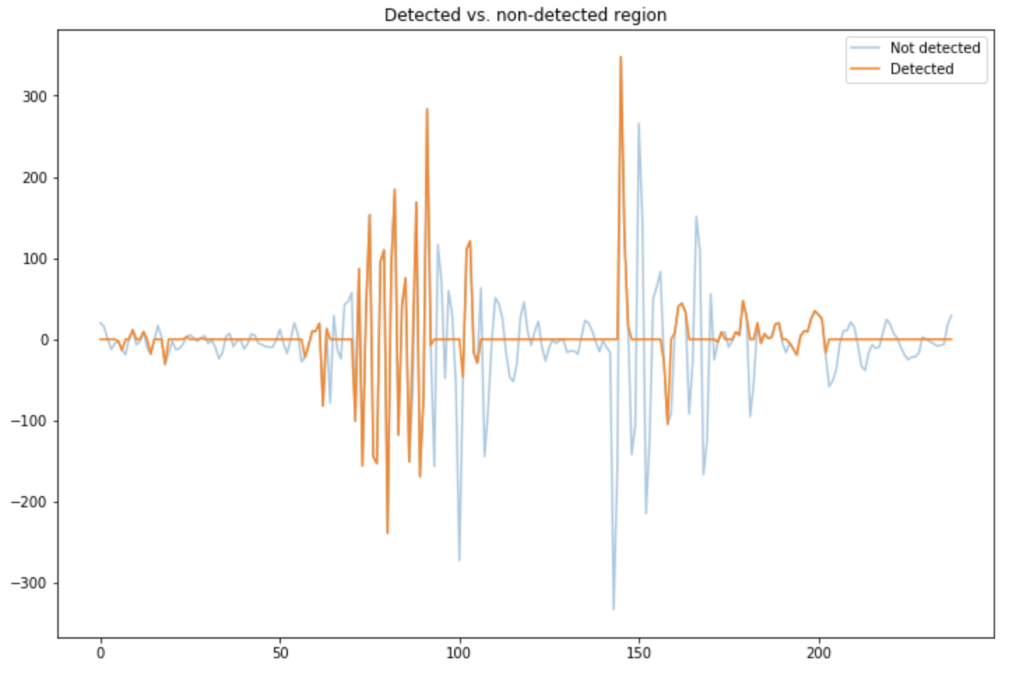
We can also compare the raw signal with moments we detected a voice:

plt.figure(figsize=(12,8))
plt.plot(np.array(mean_data), alpha=0.4, label="Not detected")
plt.plot(np.array(detected_voice) * np.array(mean_data), label="Detected")
plt.legend()
plt.title("Detected vs. non-detected region")
plt.show()

You can try to play with the speech ratio threshold and the window size to see how it affects the detection.

Smoothing the regions

The output is interesting but would require some smoothing if we want to detect smooth regions in which a user speaks. We’ll go for a median filter and apply it on the speech ratio’s list.

def _median_filter (x, k):
    assert k % 2 == 1, "Median filter length must be odd."
    assert x.ndim == 1, "Input must be one-dimensional."
    k2 = (k - 1) // 2
    
    y = np.zeros((len(x), k), dtype=x.dtype)
    y[:,k2] = x
    for i in range (k2):
        j = k2 - i
        y[j:,i] = x[:-j]
        y[:j,i] = x[0]
        y[:-j,-(i+1)] = x[j:]
        y[-j:,-(i+1)] = x[-1]
    return np.median(y, axis=1)

We can the apply it to a region

SPEECH_WINDOW = 0.5

def _smooth_speech_detection(detected_voice):
    window = 0.02
    median_window=int(SPEECH_WINDOW/window)
    if median_window % 2 == 0 : 
        median_window = median_window - 1
    median_energy = _median_filter(detected_voice, median_window)
    
    return median_energy

We can now apply this to the pipeline defined above:

speech_ratio_list = []
detected_voice = []
mean_data = []

SAMPLE_START = 0

while (SAMPLE_START < (len(data) - SAMPLE_WINDOW)):
    
    # Select only the region of the data in the window
    SAMPLE_END = SAMPLE_START + SAMPLE_WINDOW
    if SAMPLE_END >= len(data): 
        SAMPLE_END = len(data)-1
    data_window = data[SAMPLE_START:SAMPLE_END]
    mean_data.append(np.mean(data_window))
    # Full energy
    energy_freq = _connect_energy_with_frequencies(data_window)
    sum_full_energy = sum(energy_freq.values())
    
    # Voice energy
    sum_voice_energy = _sum_energy_in_band(energy_freq)
    
    # Speech ratio
    speech_ratio = sum_voice_energy/sum_full_energy
    speech_ratio_list.append(speech_ratio)
    detected_voice.append(int(speech_ratio > THRESHOLD))
    
    # Increment 
    SAMPLE_START += SAMPLE_OVERLAP
    
detected_voice = _smooth_speech_detection(np.array(detected_voice))

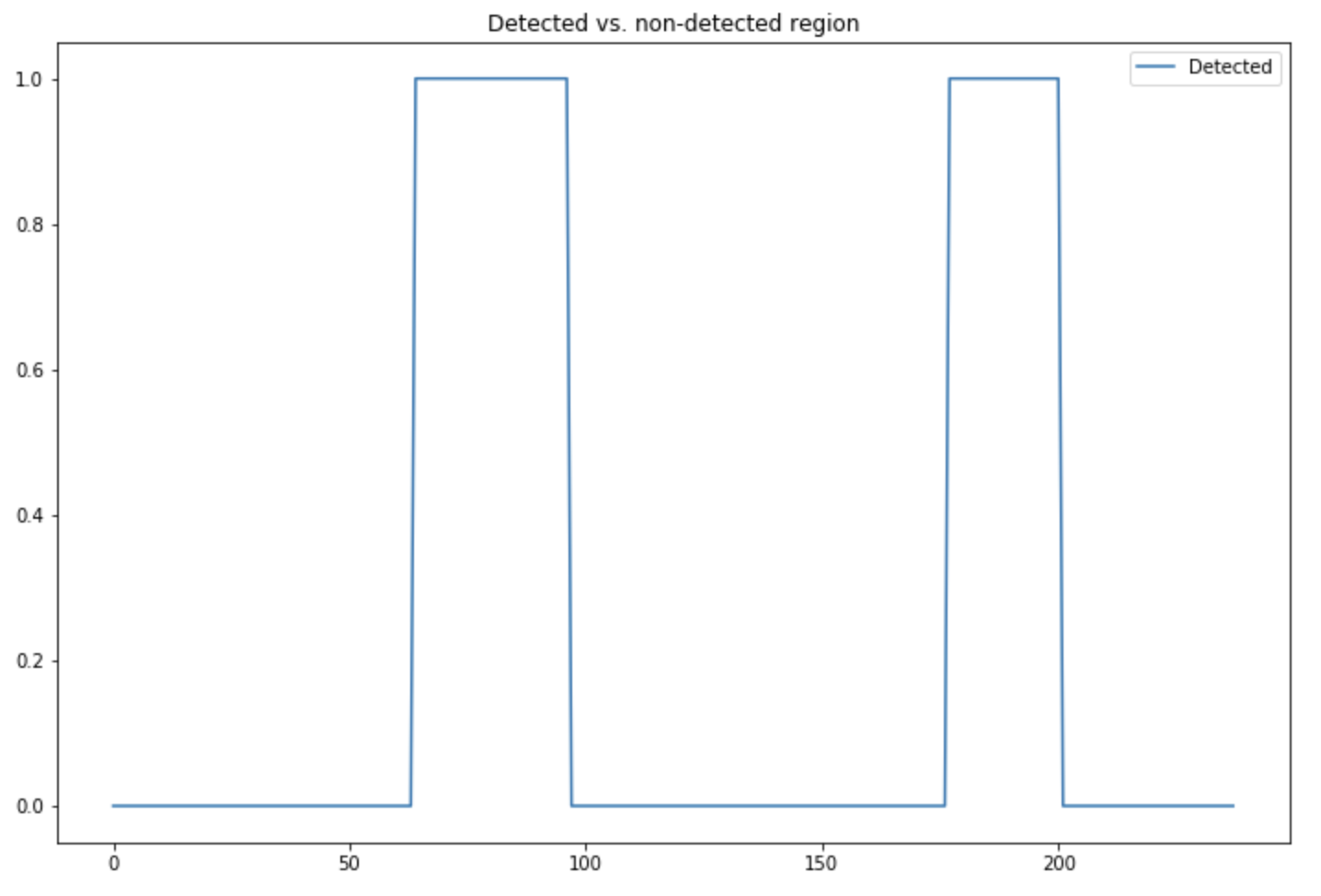
Finally, the detected regions are these ones :

plt.figure(figsize=(12,8))
plt.plot(np.array(detected_voice), label="Detected")
plt.legend()
plt.title("Detected vs. non-detected region")
plt.show()

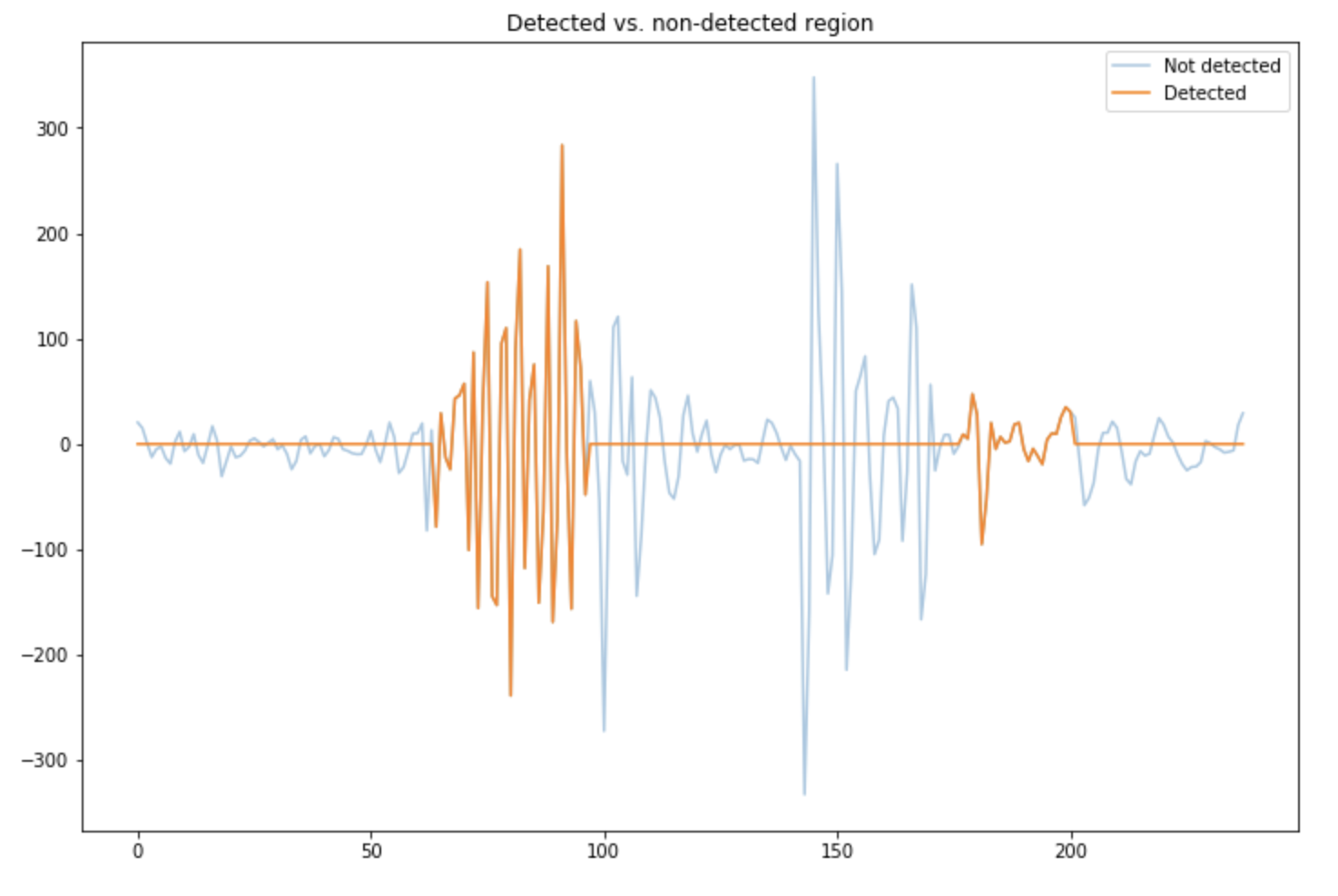
We can plot once again the regions on the raw signal in which the voice has been detected:

plt.figure(figsize=(12,8))
plt.plot(np.array(mean_data), alpha=0.4, label="Not detected")
plt.plot(np.array(detected_voice) * np.array(mean_data), label="Detected")
plt.legend()
plt.title("Detected vs. non-detected region")
plt.show()

Pros and Cons

The main advantages of this approach is that :

it runs really fast
it is easily explainable
it is simple to implement
it does not take language into account

The limits of such approach is that :

there are many hyperparameters to choose from
we must specify manually the range of frequency corresponding to a human voice
this range is not unique to humans, an an animal or a car could be interprete as a human

Conclusion: In this article, we introduced the concept of voice activity detection. In the next article, we’ll see how to create a web application to deploy our algorithm using Streamlit.

Voice Activity Detection

Maël Fabien