
Identifying a name from a first name is a hard task. Some names could be both masculine and feminine, and we usually have no other indicator than some cultural knowledge that a given name is attached to a male or a female figure.
But is it really true? Can’t we, by leveraging the letters used in names, identify whether a first name belongs to a male or a female?
Previous Work
I recently encountered an article called “Predicting the gender of Indonesian names” written by Ali Akbar Septiandri. The author, through his article, claims that he was able to predict accurately the gender of indonesian names in more than 90% of the cases.
So I started to wonder whether this was specific to Indonesian names or if I could apply it more generally to all names given in France (and not only french names).
Training Data
I used a data set that the French government published through its platform data.gouv.fr. It is an up-to-date list of the first names in France since 1900, with over 30’000 names, and can be downloaded here: https://www.data.gouv.fr/fr/datasets/ficher-des-prenoms-de-1900-a-2018/. I replaced accents by standard letters since accents nearly double the number of characters to distinguish from and do supposely not bring information on a name’s gender. I also added a similar data set with names given in the United States over the same period, of around 90’000 names, which can be downloaded here: https://data.world/howarder/gender-by-name.
My Algorithm
Start by importing the relevant packages:
import pandas as pd
import numpy as np
import matplotlib.pyplot as plt
import os

from sklearn.preprocessing import OneHotEncoder
from tensorflow.keras.preprocessing import sequence
from tensorflow.keras.models import Sequential
from tensorflow.keras.layers import Dense, Embedding, Dense, Activation, Dropout, LSTM, Bidirectional
from tensorflow.keras.callbacks import EarlyStopping, ModelCheckpoint, ReduceLROnPlateau
from sklearn.model_selection import train_test_split
from tensorflow.keras.regularizers import l2
from tensorflow.keras.utils import plot_model
from sklearn.model_selection import train_test_split
Data pre-processing
First, I pre-process the text by removing accents.
def rmv_acc(string_1):

    string_1 = string_1.replace("ç", "c")
    string_1 = string_1.replace("Ç", "C")
    string_1 = string_1.replace("à", "a")
    string_1 = string_1.replace("Ä", "A")
    string_1 = string_1.replace("ä", "a")
    string_1 = string_1.replace("À", "A")
    string_1 = string_1.replace("Â", "A")
    string_1 = string_1.replace("â", "a")
    string_1 = string_1.replace("é", "e")
    string_1 = string_1.replace("è", "e")
    string_1 = string_1.replace("É", "E")
    string_1 = string_1.replace("È", "E")
    string_1 = string_1.replace("Ë", "E")
    string_1 = string_1.replace("ë", "e")
    string_1 = string_1.replace("Ê", "E")
    string_1 = string_1.replace("ê", "e")
    string_1 = string_1.replace("û", "u")
    string_1 = string_1.replace("Û", "U")
    string_1 = string_1.replace("ü", "u")
    string_1 = string_1.replace("Ü", "U")
    string_1 = string_1.replace("ï", "i")
    string_1 = string_1.replace("Ï", "I")
    string_1 = string_1.replace("î", "i")
    string_1 = string_1.replace("Î", "I")
    string_1 = string_1.replace("Ô", "O")
    string_1 = string_1.replace("ô", "o")
    string_1 = string_1.replace("Ö", "O")
    string_1 = string_1.replace("ö", "o")
    string_1 = string_1.replace("Ù", "U")
    string_1 = string_1.replace("ù", "u")
    string_1 = string_1.replace("ÿ", "y")
    string_1 = string_1.replace("æ", "ae")
    string_1 = string_1.replace("_", " ")

    return string_1
I also convert both data sources to the same format, and load them in a single dataframe.
df = pd.read_csv('nat2018.csv', sep=";")
df = df[['sexe', 'preusuel']].drop_duplicates()
df.columns = ['gender', 'name']

def sexe(x):
    if x == 1:
        return "M"
    else:
        return "F"

df['gender'] = df['gender'].apply(lambda x: sexe(x))
columnsTitles=["name","gender"]
df=df.reindex(columns=columnsTitles)

df2 = pd.read_csv('name_gender.csv')[['name', 'gender']]

df = pd.concat([df, df2])
df['name'] = df['name'].apply(lambda x: str(x).lower())
df['name'] = df['name'].apply(lambda x: rmv_acc(x))
df = df[[len(e)>1 for e in df.name]]
df = df.drop_duplicates()

names = df['name'].apply(lambda x: x.lower())
gender = df['gender']

df.head()
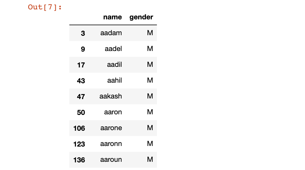
We can then take a look at the distribution of the length of names in terms of number of letters.
plt.figure(figsize=(12,8))
plt.hist([len(a) for a in names], bins=36)
plt.title("Length of the names")
plt.show()
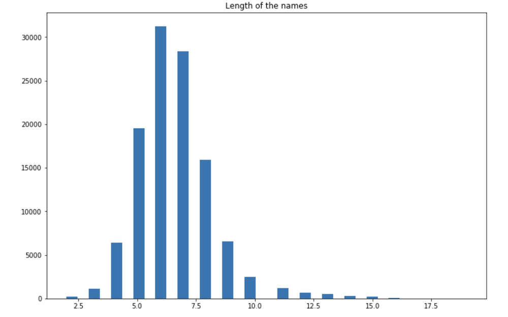
For future names to classify, we will set a threshold at 20, meaning that no name should be longer than 20 characters.
maxlen = 20
labels = 2
We can take a look at the class balance:
print("Male : " + str(sum(gender=='M')))
print("Female : " + str(sum(gender=='F')))
Male : 44580
Female : 70147
We have a bit more than 60% of female names.
I chose to explore Long Short-Term Memory (LSTMs) algorithms for this task. Such networks are usually applied at a word level, but we will apply it at a “character-level”. For this reason, we talk about character-level LSTMs.
As in LSTMs, we first must define a vocabulary which corresponds to all the unique letters encountered:
vocab = set(' '.join([str(i) for i in names]))
vocab.add('END')
len_vocab = len(vocab)
The vocabulary has a length of 30 here (taking into account special characters and all the alphabet):
{' ',
 "'",
 '-',
 'END',
 'a',
 'b',
 'c',
 'd',
 'e',
 ...}
We then create a dictionary which maps each letter of vocabulary to a number:
char_index = dict((c, i) for i, c in enumerate(vocab))
char_index
{' ': 21,
 "'": 20,
 '-': 28,
 'END': 24,
 'a': 0,
 'b': 23,
 'c': 18,
 'd': 13,
We then must create the training dataset:
X = []
y = []

# Builds an empty line with a 1 at the index of character
def set_flag(i):
    tmp = np.zeros(len_vocab);
    tmp[i] = 1
    return list(tmp)

# Truncate names and create the matrix
def prepare_X(X):
    new_list = []
    trunc_train_name = [str(i)[0:maxlen] for i in X]

    for i in trunc_train_name:
        tmp = [set_flag(char_index[j]) for j in str(i)]
        for k in range(0,maxlen - len(str(i))):
            tmp.append(set_flag(char_index["END"]))
        new_list.append(tmp)

    return new_list


X = prepare_X(names.values)

# Label Encoding of y
def prepare_y(y):
    new_list = []
    for i in y:
        if i == 'M':
            new_list.append([1,0])
        else:
            new_list.append([0,1])

    return new_list

y = prepare_y(gender)
We the split X and y into X_train, X_test, y_train and y_test.
X_train, X_test, y_train, y_test = train_test_split(X, y)
Building the model
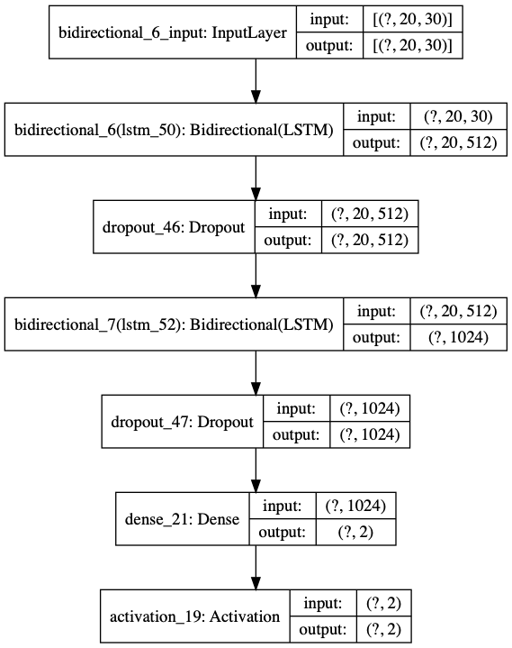
It is now time to create the model and train it. I created an architecture with a first LSTM layer, a dropout to prevent overfitting, a second LSTM layer, a second dropout, a dense layer with 2 neurons corresponding to the classification of the name as either a male or a female. I then add a sigmoid layer which outputs probabilities of belonging to one class or another. An L2 regualization has also been added on the dense layer.
I replaced LSTMs by bi-directional LSTMs to overcome the limited performance of the model. Bi-directional LSTMs depend on the whole input sequence since each layer corresponds to both a forward and a backward through time layer. This allows the output units to compute a representation that depends on both the past and the future but is most sensitive to the input values around time t. Replacing LSTMs by bi-directional ones allowed a slight validation accuracy gain.
I used Tensorflow as a back-end for a Keras architecture:
model = Sequential()
model.add(Bidirectional(LSTM(512, return_sequences=True), backward_layer=LSTM(512, return_sequences=True, go_backwards=True), input_shape=(maxlen,len_vocab)))
model.add(Dropout(0.2))
model.add(Bidirectional(LSTM(512)))
model.add(Dropout(0.2))
model.add(Dense(2, activity_regularizer=l2(0.002)))
model.add(Activation('softmax'))
model.compile(loss='categorical_crossentropy', optimizer='adam',metrics=['accuracy'])
A summary of the model is presented below:
Model: "sequential_27"
_________________________________________________________________
Layer (type)                 Output Shape              Param #
=================================================================
bidirectional_12 (Bidirectio (None, 20, 1024)          2224128
_________________________________________________________________
dropout_52 (Dropout)         (None, 20, 1024)          0
_________________________________________________________________
bidirectional_13 (Bidirectio (None, 1024)              6295552
_________________________________________________________________
dropout_53 (Dropout)         (None, 1024)              0
_________________________________________________________________
dense_24 (Dense)             (None, 2)                 2050
_________________________________________________________________
activation_22 (Activation)   (None, 2)                 0
=================================================================
Total params: 8,521,730
Trainable params: 8,521,730
Non-trainable params: 0
_________________________________________________________________
We reach 8.5 million parameters. We can also plot the model graphically:
plot_model(model, to_file='model_2.png', show_shapes=True, expand_nested=True)
We can define callbacks in Keras to:
- apply early stopping if the validation loss does not decrease anymore
- save the model which has the minimal validation loss
- reduce the learning rate on plateau if the valiadtion accuracy does not increase
callback = EarlyStopping(monitor='val_loss', patience=5)
mc = ModelCheckpoint('best_model_9.h5', monitor='val_loss', mode='min', verbose=1)
reduce_lr_acc = ReduceLROnPlateau(monitor='val_accuracy', factor=0.1, patience=2, verbose=1, min_delta=1e-4, mode='max')
It is now time to fit the model!
batch_size = 256
history = model.fit(X_train, y_train, batch_size=batch_size, epochs=35, verbose=1, validation_data =(X_test, y_test), callbacks=[callback, mc, reduce_lr_acc])
Train on 86045 samples, validate on 28682 samples
Epoch 1/35
86016/86045 [============================>.] - ETA: 0s - loss: 0.4662 - accuracy: 0.7795
Epoch 00001: saving model to best_model_9.h5
86045/86045 [==============================] - 1402s 16ms/sample - loss: 0.4662 - accuracy: 0.7795 - val_loss: 0.4304 - val_accuracy: 0.8070
Epoch 2/35
86016/86045 [============================>.] - ETA: 0s - loss: 0.3972 - accuracy: 0.8249
Epoch 00002: saving model to best_model_9.h5
...
The training takes 2 to 3 hours on CPUs, and reaches the early stopping at around 18 epochs. We can plot the training and validation accuracy curves:
plt.figure(figsize=(12,8))
plt.plot(history.history['accuracy'])
plt.plot(history.history['val_accuracy'])
plt.title('Model accuracy')
plt.ylabel('Accuracy')
plt.xlabel('Epoch')
plt.legend(['Train', 'Test'], loc='upper left')
plt.show()
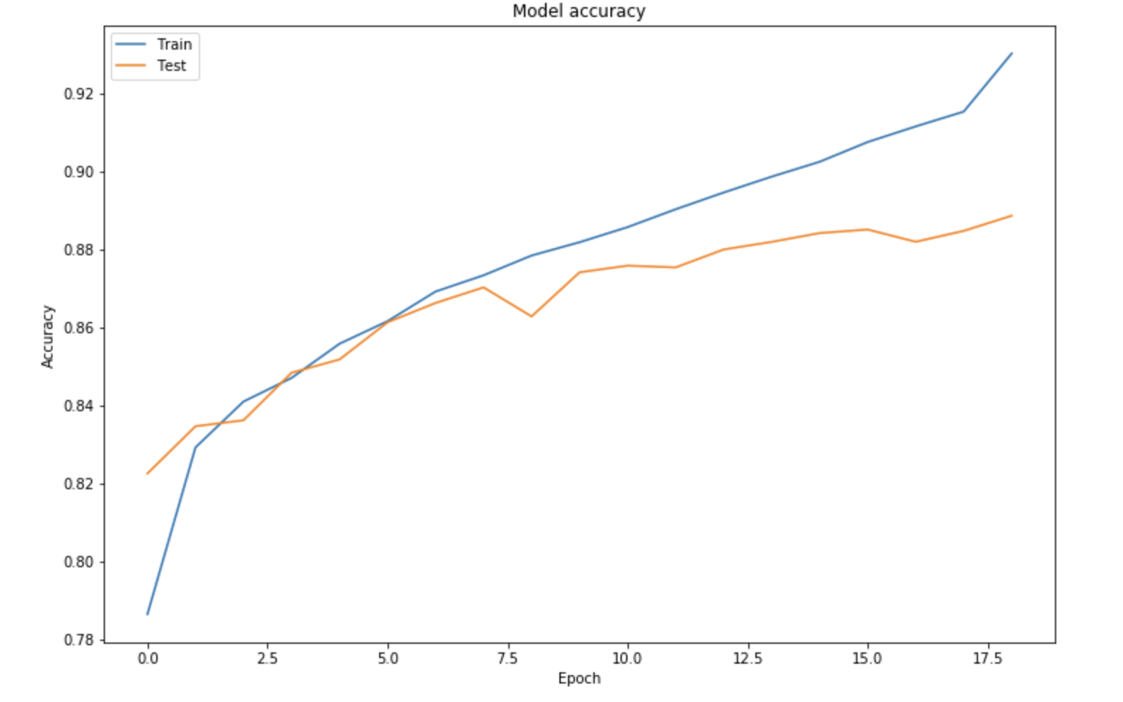
We reach a validation accuracy of 89.5% but notice a slight overfitting, although drop out, L2-regularization and reduction of learning rate had been applied.
Making predictions
Let’s make predictions using the trained model now!
We first define new names, and process them:
new_names = ["mael", "jenny", "marc"]
X_pred = prepare_X([rmv_acc(e) for e in new_names])
Then, we make the predictions:
prediction = model.predict(X_pred)
prediction
Which returns :
array([[0.3685085 , 0.6314915 ],
       [0.14170532, 0.85829467],
       [0.8759549 , 0.12404503]], dtype=float32)
To make it more understandable, we create a function which maps this to labels (M or F), or N (for neutral) if the probability is not high enough:
def pred(new_names, prediction, dict_answer):
    return_results = []
    k = 0
    for i in prediction:
        if max(i) < 0.65:
            return_results.append([new_names[k], "N"])
        else:
            return_results.append([new_names[k], dict_answer[np.argmax(i)]])
        k += 1
    return return_results
If we run this on the predictions above:
pred(new_names, prediction, dict_answer)
Which returns:
[['mael', 'N'], ['jenny', 'F'], ['marc', 'M']]
The outcome is good, since Mael in French can be used for both Males and Females, Jenny is a female name and Marc a male name.
Conclusion
In conclusion, we covered in this article a method to apply character-level bi-directional LSTMs for gender classification from first names. We are slightly below the accuracy of the authors of the papers “Predicting the gender of Indonesian names” but we face a large names database of over 120’000 names given in France and in the US.