
To analyze text and run algorithms on it, we need to embed the text. The notion of embedding simply means that we’ll convert the input text into a set of numerical vectors that can be used into algorithms. In this article, we’ll focus on Word2Vec, a state of the art embedding method, that embeds each word individually.
For the sake of clarity, we’ll call a document a simple text, and each document is made of words, which we’ll call terms.
The techniques we are about to cover were first introduced by Google in 2013. The original paper can be found here. Among the authors, you’ll probably recognize Jeff Dean or Tomas Mikolov.
I. Why should we embed words?
Embedding, as stated above, is used to create feature vectors from words. The idea is to encode their meaning and allow us to calculate a similarity score for any pair of words for example.
What can we do with an embedded corpus?
- determine similarity scores between documents for a search engine, using cosine similarity for example
- identify topics of the documents
- build a recommender system to suggest other movies based on the synopsis
- machine translation to identify that “Au revoir” and “Goodbye” actually mean the same thing
II. General Word Embedding Principles
In Word Embedding in general, we want a model to learn to associate a vector to a word but embedding the semantic links between words, using the word context.
The main hypothesis between word embedding is the distributional semantics. We suppose that 2 words occurring in the same context have semantic proximity.
We need as an input a large dataset of texts, and by training a model, we expect to get for each word of the vocabulary, a vector of a pre-determined size, say 300, that looks like this :
dog = [0.2854, 0.8711, -0.5217, 0.1281, ...]
We generally use Neural Networds to encode those dimensions, in methods such as Word2Vec. These representations are very good at encoding dimensions of similarity. Indeed, in the embedding space, the following relations should more or less hold :
- Syntactically : \(x_{orange} - x_{oranges} = x_{train} - x_{trains} = x_{phone} - x_{phones}\)
- Semantically : \(x_{queen} - x_{woman} = x_{king} - x_{man}\)
The context of a word is the set of the C surrounding words. Words on the left of the word we’d like to embed are called the left context. Words on the right are called the right context. The order of the words within the context has however no importance.
For example, say that we want to embed the word “dog”, and encounter the following sentence :
I am walking my dog with Julie
If we take a 2 left-right context, i.e 2 words on the left, and 2 words on the right, the context will be :
{Walking, my, with, Julie}
Within the context of the embedding of the dog, the words Walking and Julie will be relevant.
III. The Word2Vec Skip-gram model
Word2Vec works pretty much as an auto-encoder. We will train on one side a neural network to perform a certain task on one side, and on the other side to undo it to get back to the original result.
There are two variants of the Word2Vec paradigm – skip-gram and CBOW. The skip-gram variant takes a target word and tries to predict the surrounding context words, while the CBOW (continuous bag of words) variant takes a set of context words and tries to predict a target word. We’ll start by focusing on the Skip-gram model, and develop the C-BoW in a further article.
General idea
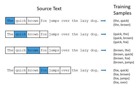
First of all, we need to define the list of vocabulary. The task we’ll teach our model to do is to learn the probability that two words are “nearby” within a text. For each “target” word among our vocabulary, we do that by :
- defining a window size, i.e. the context of the word
- picking randomly a word within the window size around the target word
- counting the number of times they appear together
- applying softmax activation to create probabilities
The output probabilities are a measure of how likely it is that these 2 words appear together.
We give the network as an entry the pairs of words. To add randomness into the process, the window size in the training process is chosen randomly, between 1 and the specified window size.
If we have 5’000 words of vocabulary and we fit our model on it, the output of the network should be a 5’000 * 5’000 matrix, and within each position the probability that these words appear together.
Model details
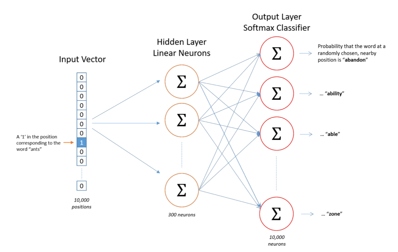
The model is made of a single hidden layer and an output layer with a softmax classifier.
-
The input of the model is a vector that has the size of the vocabulary, 0’s everywhere except for a 1 at the position of the word we’d like to embed.
-
The output of the model is a softmax layer that has the size of the vocabulary, and for each word, the probability that this word will be observed in the context of the input word. Softmax transforms to map the output as probabilities that sum to 1 :
- The hidden layer helps to choose the size of the vectors we’ll later be using. If we set the hidden layer size to 500, the hidden layer will be a weight matrix of the size of the vocabulary, say 15’000 rows times 500 columns. The hidden layer in this model is mainly operating a lookup-table, i.e selecting the row corresponding to the word vector. Google, for its Word2Vec, has used 300 dimensions for example.
By multiplying a feature vector of “dog” with an output layer of “walking”, what we’re computing here is the probability that if we pick a word randomly around “dog”, this word is “walking” for example.
If two words are different be happen in similar contexts, our model will learn similar word vectors for these words, i.e. “engine” and “transmission”.
All we need to do once the model has been trained is to drop the output layer. Indeed, we are only interested in the vector representation of the words, and as in auto-encoder, the second part of the network will not be used.
Limits of the Skip-gram
The Skip-Gram model must compute a huge number of weights. For a vocabulary size of 10’000 words and 500 features, we would have 5 million weights in the hidden layer and the output layer. We also need a huge number of training data (typically counting in billions at that point). Since companies like Google train those models on the entire Web (or close), the number of weights to compute is just enormous.
It has been shown recently that training a single Word Embedding Model can produce as much Co2 as 5 cars in their entire lifetime. See this article for more information.
The training becomes pretty much impossible, which is the reason why the authors of Word2Vec have developed a second version called Continuous Bag-Of-Words that contains several tweaks to make the training faster.
Performance improvements of Word2Vec Skip-Gram model
Subsampling frequent words
When we create training samples :
- words such as “the”, “my”, “a”… don’t bring much information
- we’ll end up with too many samples containing these stop words
The authors propose a sampling rate which states whether we should keep a word or not. \(P(w_i)\) describes the probability of keeping a word :
\[P(w_i) = ( \sqrt{ \frac {z(w_i)} {0.001}} + 1 ) \times \frac {0.001} {z(w_i)}\]Where \(z(w_i)\) is the fraction of the total words in the corpus that the word \(w_i\) represents.
The value 0.001 is proportional to the fraction of the most frequent words we’ll remove. By training our model on the whole of Wikipedia, setting the sample to 0.001 would only remove 27 words. However, these 27 words represent up to 33% of all words on Wikipedia. These words include :
- the
- of
- and
- in
- to
- was
- is
- …
By subsampling, we can reduce this 33% ratio to 22%, since the probabilities to keep those words are rather low.
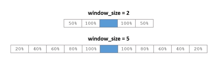
Context Position Weighting
In the most Word2Vec most standard implementation, we randomly shrink the size of the context window. We want to weight the context words according to how close they are to the target word. This is done in the random shrinking. Indeed, for different maximum window sizes, the percentage that a given box is included in a context is the following :
Negative sampling
By training our neural network, we adjust the neuron weights for each input data. However, we have to modify all weights at each step, i.e. billions of weight for each training sample.
In negative sampling, we only modify a small percentage of the weights at each step. Indeed, we will modify the weights of “negative samples”, i.e a list of 5 to 20 words that we will take as inputs along with the target word.
We want the neuron to output 0 for all the negative samples that we added to our target word. By doing this, instead of selecting the whole vocabulary size, we select typically 10+1=11 words out of a vocabulary size of 10’000 for example. This is a drastic drop in the overall amount of computations required.
We are doing kind of a random pick of the words to select in the negative samples, with slight modification since we raise an element to a certain power (this was chosen empirically in the original paper).
\[P(w_i) = \frac {f(w_i)^{\frac{3}{4}}} {\sum_j(f(w_j)^{\frac{3}{4}})}\]Where \(f(w_i)\) is the number of times a given word appears in the corpus, and the denominator is the total number of words in the corpus.
Conclusion : And this is it. We have covered the main concepts of the Skip-Gram version of Word2Vec. I hope this introduction to Bag-Of-Words in NLP was helpful. Don’t hesitate to drop a comment if you have a comment.
Sources :
- NLP class at Telecom ParisTech
- The Inner Workings of Word2Vec by Chris McCormick, which I highly recommend