To analyze text and run algorithms on it, we need to represent the text as a vector. The notion of embedding simply means that we’ll convert the input text into a set of numerical vectors that can be used into algorithms. There are several approaches that I’ll describe in the next articles. In this article, we’ll start with the simplest approach: Bag-Of-Words.

For the sake of clarity, we’ll call a document a simple text, and each document is made of words, which we’ll call terms.

Both Bag-Of-Words and TF-IDF methods represent a single document as a single vector.

I. What is Bag-Of-Words?

1. Bag-Of-Words

When we use Bag-Of-Words approaches, we apply a simple word embedding technique. Technically speaking, we take our whole corpus that has been preprocessed, and create a giant matrix :

the columns correspond to all the vocabulary that has ever been used with all the documents we have at our disposal
the lines correspond to each of the document
the value at each position corresponds to the number of occurrence of a given token within a given document

Bag-Of-Words (BOW) can be illustrated the following way :

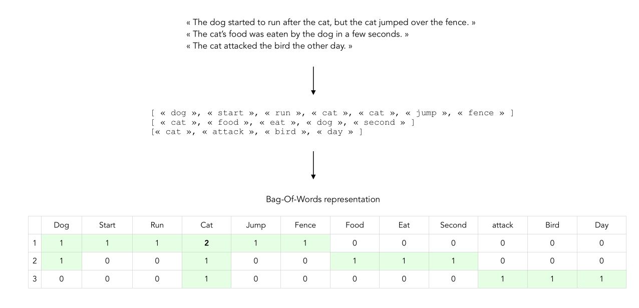
The number we fill the matrix with are simply the raw count of the tokens in each document. This is called the term frequency (TF) approach.

\[tf_{t,d} = f_{t,d}\]

where :

the term or token is denoted \(t\)
the document is denoted \(d\)
and \(f\) is the raw count

This approach is however not so popular anymore. What are the limitations implied by this model?

the more frequent a word, the more importance we attach to it within each document which is logic. However, this can be problematic since common words, like cat or dog in our example, do not bring much information about the document it refers to. In other words, words that appear the most are not the most interesting to extract information from a document.
we could leverage the fact that the words that appear rarely bring a lot of information on the document it refers to

2. Term Frequency Inverse Document Frequency (TF-IDF)

For the reasons mentioned above, the TF-IDF methods were quite popular for a long time, before more advanced techniques like Word2Vec or Universal Sentence Encoder.

In TF-IDF, instead of filling the BOW matrix with the raw count, we simply fill it with the term frequency multiplied by the inverse document frequency. It is intended to reflect how important a word is to a document in a collection or corpus.

\[tfidf_{t,d} = f_{t,d} \times invf_{t,d}\] \[= f_{t,d} \times ( \log \frac {M} {df_t})\]

Where :

the term frequency \(f_{t,d}\) counts the number of occurences of \(t\) in \(d\).
the document frequency \(df_t\) counts the number of documents that contain the word \(t\)
M is the total number of documents in the corpus

The TF-IDF value grows proportionally to the occurrences of the word in the TF, but the effect is balanced by the occurrences of the word in every other document (IDF).

3. Measuring the similarity between documents

In the vector space, a set of documents corresponds to a set of vectors in the vector space. The cosine similarity descrives the similariy between 2 vectors according to the cosine of the angle in the vector space :

\[cos_{sim}(d_1, d_2) = \frac { \bar{V}(d_1) \bar{V}(d_2) } { \mid \bar{V}(d_1) \mid \mid \bar{V}(d_2) \mid }\]

II. Implementation in Python

Let’s now implement this in Python. The first step is to import NLTK library and the useful packages :

import numpy as np
import pandas as pd
import re
from sklearn.feature_extraction.text import CountVectorizer, TfidfVectorizer
from nltk import wordpunct_tokenize, WordNetLemmatizer, sent_tokenize, pos_tag
from nltk.corpus import stopwords as sw, wordnet as wn
from keras.preprocessing.text import Tokenizer
from keras.preprocessing.sequence import pad_sequences
import string 

1. Preprocessing per document within-corpus

The pre-processing will be similar to the one developed in the previous article. We’ll use the preprocess function. This pipeline is only an example that happened to suit my needs on several NLP projects. It has many limitations, including the fact that it only handles English vocabulary.

We will work with some data from the South Park series. The data set is made of all the conversations of all the characters in South Park. The data can be downloaded here. We’ll focus here on the first 1000 rows of the data set.

df = pd.read_csv('All-Seasons.csv')['Line'][:1000]
df.head()

         You guys, you guys! Chef is going away. \n
                        Going away? For how long?\n
                                         Forever.\n
                                  I'm sorry boys.\n
  Chef said he's been bored, so he joining a gro...
...

Let’s now apply our preprocessing to the data set :

df, vocab = preprocess(list(df))

The new data set will now look like this :

[['you', 'guy', 'you', 'guy', 'chef', 'be', 'go', 'away'],
['go', 'away', 'for', 'how', 'long'],
['forever'],
...

And the vocabulary, which has size 1569 here, looks like this :

vocab

...
'aaaah',
'able',
'aboat',
'aborigine',
'abort',
'about',
'academy',
'acceptance',
'acid',
'ack',
'across',
'act'
...

Let us now define the BOW function for Term Frequency! Note that the following implementation is by far not optimized.

def generate_bow(allsentences):    
    # Define the BOW matrix
    bag_vector = np.zeros((len(allsentences), len(vocab)))
    # For each sentence
    for j in range(len(allsentences)):
        # For each word within the sentence
        for w in allsentences[j]:
            # For each word within the vocabulary
            for i,word in enumerate(vocab):
                # If the word is in vocabulary, add 1 in position
                if word == w: 
                    bag_vector[j,i] += 1
    return bag_vector

We can then apply the BOW function to the cleaned data :

bow = generate_bow(df)

It generates the whole matrix for the 1000 rows in 1.42s.

array([[0., 0., 0., ..., 0., 0., 0.],
[0., 0., 0., ..., 0., 0., 0.],
[0., 0., 0., ..., 0., 0., 0.],
...

2. BoW in Sk-learn

So far, we used a self-defined function. As you might guess, there is a Scikit-learn way to do this :)

You might need to modify a bit the preprocessing function. Indeed, the only thing you’ll want to modify is when you append the lemmatized tokens to the clean_document variable :

cleaned_document.append(' '.join(lemmatized_tokens))

After which the application in Sk-learn is straightforward :

df = preprocess(list(df))
vectorizer = CountVectorizer()
X = vectorizer.fit_transform(df).toarray()

The count vectorizer runs in 50ms.

3. TF-IDF in Sk-learn

We can apply TF-IDF in Sk-learn as simply as this :

vectorizer = TfidfVectorizer()
X = vectorizer.fit_transform(df).toarray()

III. Limits of BoW methods

The reason why BOW methods are not so popular these days are the following :

the vocabulary size might get very, very (very) large, and handling a sparse matrix with over 100’000 features is not so cool. If you want to control it, you should set a maximum document length or a maximum vocabulary length. Both imply large biases.
the order of the words in the sentence does not matter, which is a major limitation

For example, the sentences: “The cat’s food was eaten by the dog in a few seconds.” does not have the same meaning at all than “The dog’s food was eaten by the cat in a few seconds.”. To overcome the dimension’s issue of BOW, it is quite frequent to apply Principal Component Analysis on top of the BOW matrix.

In the next article, we’ll see more evolved techniques like Word2Vec which perform much better and are currently close to state of the art.

Conclusion : I hope this quick introduction to Bag-Of-Words in NLP was helpful. Don’t hesitate to drop a comment if you have a comment.

From text to vectors with BoW and TF-IDF

Maël Fabien