
Linear Discriminant Analysis is a generative model for classification. It is a generalization of Fisher’s linear discriminant. LDA works on continuous variables. If the classification task includes categorical variables, the equivalent technique is called the discriminant correspondence analysis.
The goal of Linear Discriminant Analysis is to project the features in higher dimension space onto a lower-dimensional space to both reduce the dimension of the problem and achieve classification.
Key ideas
- Generative Model that tries to estimate \(P (X = x \mid Y = 1)\) and \(P (X = x \mid Y = -1)\)
- Used for classification through dimension reduction
- Requires continuous variables
- Relies on normality assumption for \(P(X \mid Y = 1)\) and \(P(X \mid Y = 0)\)
- Requires homoscedasticity and full rank covariances
Concept
Consider a simple problem in which we want to decide whether a drug should be given to patients or not. Our features will be the gene expressions, and we will have 2 labels, for patients for which the drug worked, and for which it did not.
In PCA, we are interested in genes with the largest variations. In LDA, we are interested in maximizing the separability between the 2 known groups to make better decisions.
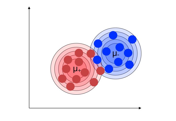
We’ll illustrate how we can improve the separability by this simple example. We suppose that we have 2 features, one for each gene. This means that we can plot the graph on a 2D plane.
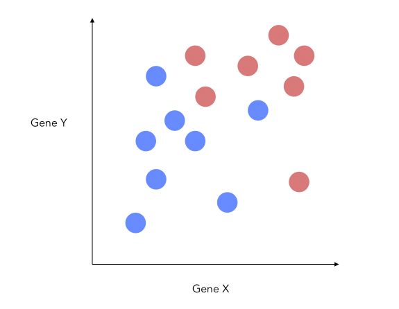
How can we reduce the dimension of this problem to 1D ?
A bad way to approach this problem would be to project on the X-axis.
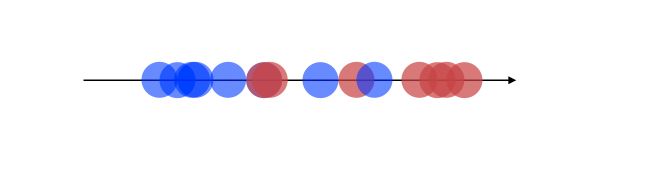
This would imply losing a lot of information from the Y-axis. what LDA does is that it projects the data onto a new axis in a way to maximize the separation between the 2 categories.
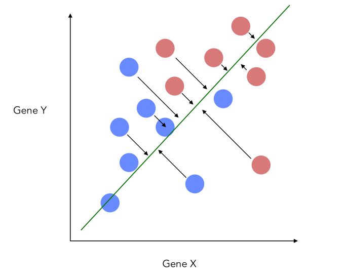
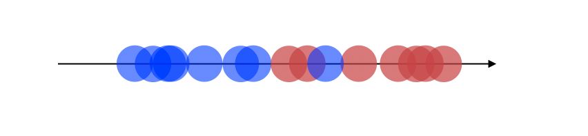
The projection, therefore, looks like this now, which is a good improvement :
How is this new axis created ?
- The new axis should maximize the distance between the two means :
- The new axis should minimize the variation, i.e scatter within each category
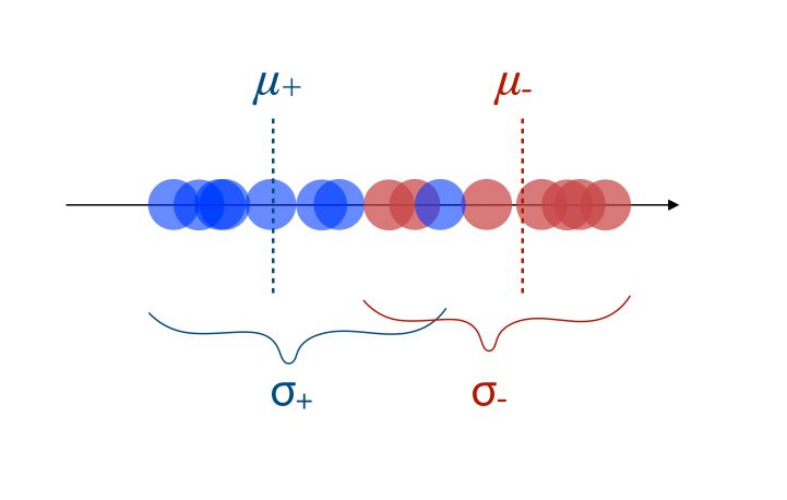
Both of the criteria can be optimized using the following ratio :
\[\frac { (\mu_+ - \mu_-)^2 } {( \sigma_+ + \sigma_-)} = \frac { d^2 } {( \sigma_+ + \sigma_-)}\]The numerator should ideally be large, and the numerator should be small. If we have 3 dimensions or more, the process remains the same!
If we have 3 categories, the process pretty much remains the same. We compute the distance to a central point and maximize the distance with respect to it.
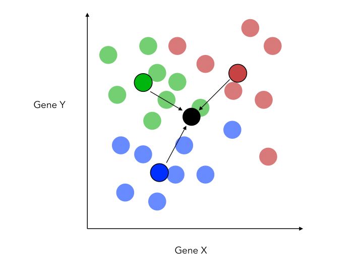
The new criteria is now :
\[\frac { {d_{1-2}}^2 + {d_{1-3}}^2 + {d_{2-3}}^2 } {( \sigma_1 + \sigma_2 + \sigma_3)}\]Another thing that changes when adding this class is that we do now project on a new place, not a single axis. This is because the 3 central points for each category define a plane. We can now build new X and Y axis, optimized for classification.
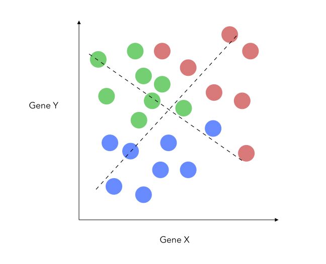
Being able to draw the data on 2 axes is interesting if we have an initial high dimensional problem. Once we redefined our X and Y axis, it is really easy to apply fit a linear regression on top! And voilà, this is the LDA!
Theory
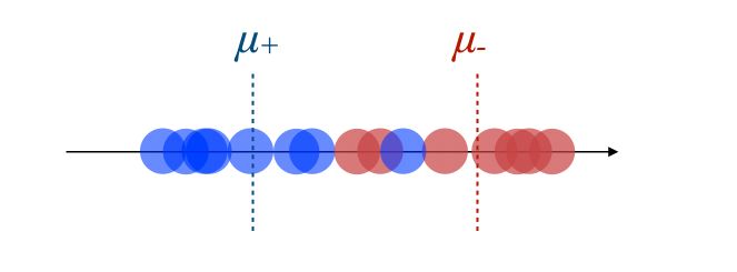
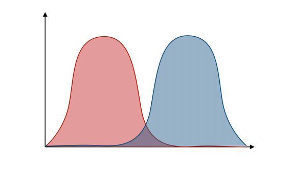
Back to our example with 2 classes. We would like to find the two underlying marginal distributions.
We’ll define the distributions of the 2 classes :
- \(G = L(X \mid Y=1)\) distribution of the class 1
- \(H = L(X \mid Y=-1)\) distribution of the class -1
We can plot the probability densities :
The LDA relies on some strong hypothesis which we’ll explicit now.
Gaussian marginal distributions
- \[G = N(\mu_+, \sigma_+)\]
- \[H = N(\mu_-, \sigma_-)\]
where :
\[N(\mu, \sigma^2) = \frac {1} {\sqrt {2 \pi \sigma^2}} e^{ \frac {-1} {2 \sigma^2} {(x-\mu)^2}}\]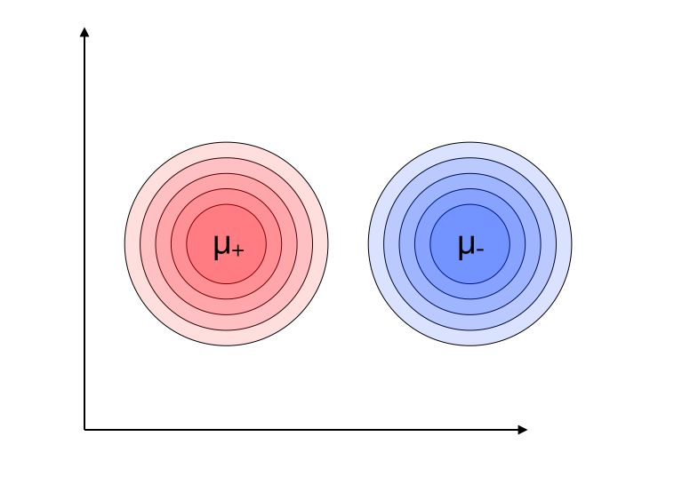
Homoscedasticity
LDA should be used when the covariance matrices are equal among the 2 classes :
\[\sigma_+ = \sigma_- = \sigma\]Learning process
To understand the intuition behind how LDA works, we can define a likelihood ratio :
\[\phi(X) = \frac { \delta G} { \delta H} (x) = \frac {P(X = x \mid Y = 1)} {P(X = x \mid Y = -1)}\]Using Bayes’ theorem :
\[\phi(X) = \frac {P(Y = 1 \mid X = x) \frac {P(X=x)} {P(Y=1)}} {P(Y = -1 \mid X = x) \frac {P(X=x)} {P(Y=-1)}}\] \[\phi(X) = \frac { \frac { P(Y = 1 \mid X = x) } { P(Y=1) } } { \frac { P(Y = -1 \mid X = x) } { P(Y=-1) } }\]We can re-define \(P(Y=1)\) as \(p\) and \(P(Y=1 \mid X = x)\) as the prior probability \(\eta(x)\).
\[\phi(X) = \frac {1-p} {p} \frac {\eta(x)} {1-\eta(x)}\]We can easily isolate the prior probability \(\eta(x)\) :
\[\eta(x) = \frac { p \phi(x) } {(1-p) + p \phi(x)}\]Computation
How do we find the parameters of the model? How does the learning process work?
\[\eta(x) = \frac { e^{ ( \frac {-1} {2} ( x - \mu_+ )^T \sigma^{-1} (x-\mu_+) ) } } {e^{ ( \frac {-1} {2} (x - \mu_-)^T \sigma^{-1} (x- \mu_- ) ) } }\] \[= e^{ ( \frac {-1} {2} (x-\mu_+)^T \sigma^{-1} (x-\mu_+) + \frac {-1} {2} (x-\mu_-)^T \sigma^{-1} (x-\mu_-) ) }\] \[= e^{ (x^T \sigma^{-1} {\mu_+}^T - \frac {1} {2} \mu_+ \sigma_{-1} \mu_- - x^T \sigma^{-1} \mu_- + \frac {1} {2} {\mu_-}^T \sigma_{-1} \mu_- ) }\]If \(\eta(x) > \frac {1} {2}\), then \(\phi(x) ≥ \frac {1-p} {p}\) . This means that :
\[x^T \sigma^{-1} (\mu_+ - \mu_-) + \frac {1} {2} ( {\mu_+}^T \sigma_{-1} \mu_- {\mu_+}^T \sigma^{-1} \mu_+) ≥ log \frac {p} {1-p}\]Which can be re-written as :
\[\alpha + \beta^T x ≥ 0\]Where :
\[\beta = \sigma^{-1}(\mu_+ - \mu_-)\] \[\alpha = \frac {1} {2} ({\mu_-}^t \sigma^{-1} \mu_- - {\mu_+}^t \sigma^{-1} \mu_+) - \log \frac {p} {1-p}\]This should remind you of the ratio to optimize we defined in the first part of the article! The parameter \(\alpha\) and \(\beta\) are the parameters of the linear regression fitted on the modified axis plane.
Parameter estimation
The question now becomes : How can we estimate \(\alpha\) and \(\beta\) ? By Maximum Likelihood, we obtain the following :
\[\hat{p} = \frac { \sum_i I_{y_i = 1} } { n} = \frac {n_+} {n}\] \[\hat{\mu_+} = \frac { 1} {n_+} \sum_{Y_i = 1} X_i\] \[\hat{\mu_-} = \frac {1} {n_-} \sum_{Y_i = -1} X_i\] \[\hat{\sigma} = \frac {n_+} {n} \hat{\sigma_+} + \frac {n_-} {n} \hat{\sigma_-}\]We then simply replace those values to find \(\hat{\alpha}\) and \(\hat{\beta}\).
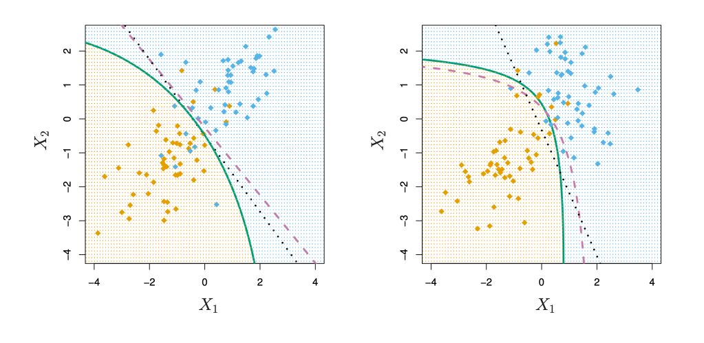
Quadratic Discriminant Analysis (QDA)
So far, we supposed that the class variance had to be the same : \(\sigma_+ = \sigma_- = \sigma\). If we relax this hypothesis, we obtain the QDA, where \(\sigma_+ ≠ \sigma_-\).
Conclusion : I hope this introduction to LDA was helpful. Let me know in the comments if you have any question.