
Bayesian Hyperparameter Optimization is a model-based hyperparameter optimization. On the other hand, GridSearch or RandomizedSearch do not depend on any underlying model.
What are the main advantages and limitations of model-based techniques? How can we implement it in Python?
Bayesian Hyperparameter Optimization
Sequential model-based optimization (SMBO)
In an optimization problem regarding model’s hyperparameters, the aim is to identify :
\[x^* = argmin_x f(x)\]where \(f\) is an expensive function.
Depending on the form or the dimension of the initial problem, it might be really expensive to find the optimal value of \(x\). Hyperparameter gradients might also not be available. Suppose that we know all the parameters distribution. We can represent for every hyperparameter, a distribution of the loss according to its value.
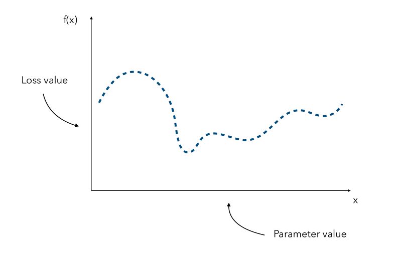
Since the curve is not known, a naive approach would be the pick a few values of x and try to observe the corresponding values f(x). We would then pick the value of x that gave the smallest value.
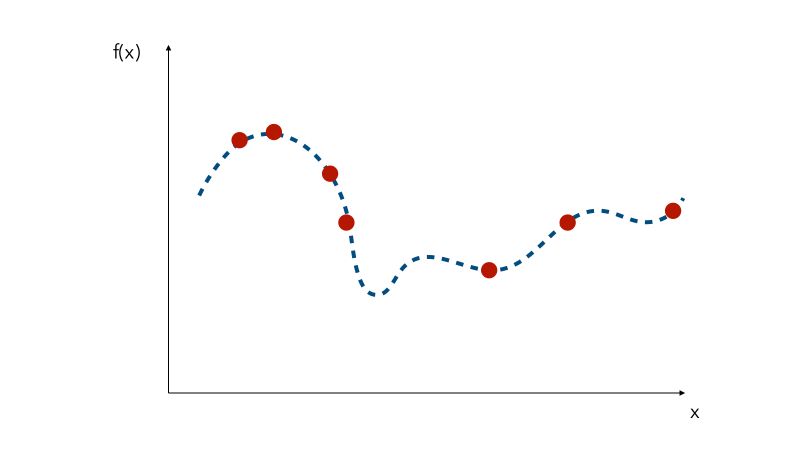
We can pick values randomly, but other common methods are :
- quasi-random sampling
- Latin hypercube sampling
Probabilistic Regression Models
We try to approximate the underlying function using only the samples we have. This can essentially be done in 3 ways :
- using Gaussian Process (GP)
- using Random Forests
- using Tree Parzen Estimators (TPE)
Gaussian Process (GP)
We suppose that the function \(f\) has a mean \(\mu\) and a covariance \(K\), and is a realization of a Gaussian Process. The Gaussian Process is a tool used to infer the value of a function. Predictions follow a normal distribution. Therefore :
\[p(y \mid x, D) = N(y \mid \hat{\mu}, {\hat{\sigma}}^2)\]We use that set of predictions and pick new points where we should evaluate next. We can plot a Gaussian Process between 4 samples this way :
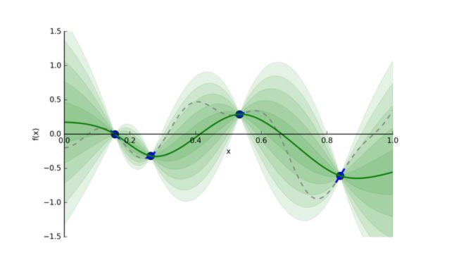
The green areas represent confidence intervals.
From that new point, we add it to the samples and re-build the Gaussian Process with that new information… We keep doing this until we reach the maximal number of iterations or the limit time for example.
Random Forests
Another choice for the probabilistic regression model is an ensemble of regression trees. This is used by Sequential Model-based Algorithm Configuration library (SMAC).
We still suppose that \(N(y \mid \hat{\mu}, {\hat{\sigma}}^2)\) is Gaussian.
We choose the parameters \(hat{\mu}, \hat{\sigma}\) as the empirical mean and variance of the regression values.
\[\hat{\mu} = \frac {1} { \mid B \mid } \sum_{r \in B} r(x)\] \[{\hat{\sigma}}^2 = \frac {1} { \mid B \mid - 1 } \sum_{r \in B} ( r(x) - \hat{\mu} )^2\]By their structure, Random Forests allow the use of conditional variables, which is a nice feature.
Tree Parzen Estimators (TPE)
TPE does not define a predictive distribution. Instead, it creates two hierarchical processes, \(l(x)\) and \(g(x)\) acting as generative models for all domain variables. These processes model the domain variables when the objective function is below and above a specified quantile \(y^*\).
\(p(x \mid y, D) = l(x)\) if \(y < y^*\), else \(g(x)\)
Gaussian processes and random forests, in contrast, model the objective function as dependent on the entire joint variable configuration.
Parzen estimators are organized in a tree structure, preserving any specified conditional dependence and resulting in a fit per variable for each process \(l(x), g(x)\). With these two distributions, one can optimize a closed-form term proportional to the expected improvement
TPE naturally supports domains with specified conditional variables.
Acquisition function
How do we pick the point to know where we should evaluate next?
- Pick points that yield, on the approximated curve, a low value.
- Pick points in areas we have less explored.
There is an exploration/exploitation trade-off to make. This tradeoff is taken into account in an acquisition function.
The acquisition function is defined as :
\[A(x) = \sigma(x) ( \gamma(x) \Phi( \gamma(x)) + N (\gamma(x)))\]where :
- \[\gamma(x) = \frac { f(x^c) - \mu(x)} {\sigma(x)}\]
- \(f(x^c)\) the current guessed arg min, \(\mu(x)\) the guessed value of the function at
x, and \(\sigma(x)\) the standard deviation of output atx. - \(\Phi(x)\) and \(N(x)\) are the CDF and the PDF of a standard normal
We then compute the acquisition score of each point, pick the point that has the highest activation, and evaluate \(f(x)\) at that point, and so on…
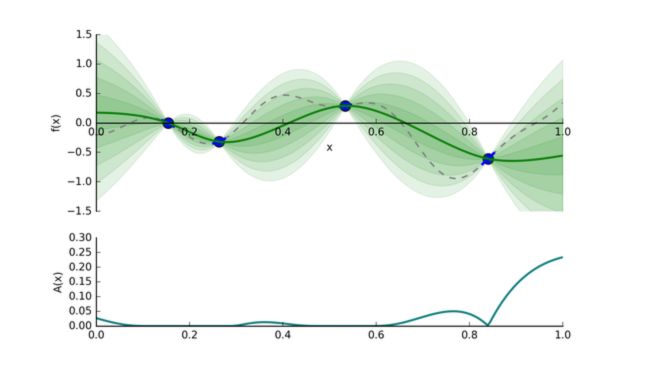
In this example, we would move to the extreme value on the right, at \(x = 1\).
The process can be illustrated in the following way :
This is the essence of bayesian hyperparameter optimization!
Advantages of Bayesian Hyperparameter Optimization
Bayesian optimization techniques can be effective in practice even if the underlying function \(f\) being optimized is stochastic, non-convex, or even non-continuous.
Bayesian optimization is effective, but it will not solve all our tuning problems. As the search progresses, the algorithm switches from exploration — trying new hyperparameter values — to exploitation — using hyperparameter values that resulted in the lowest objective function loss.
If the algorithm finds a local minimum of the objective function, it might concentrate on hyperparameter values around the local minimum rather than trying different values located far away in the domain space. Random search does not suffer from this issue because it does not concentrate on any values!
Implementation in Python
Several softwares implement Gaussian Hyperparameter Optimization.
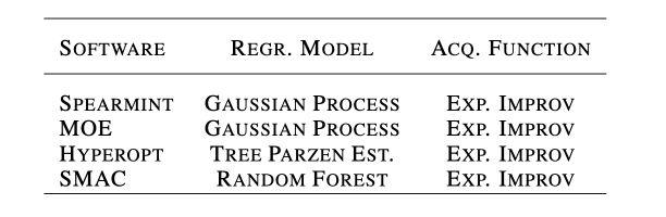
We’ll be using HyperOpt in this example.
The Data
We’ll use the Credit Card Fraud detection, a famous Kaggle dataset that can be found here.
The datasets contain transactions made by credit cards in September 2013 by European cardholders. This dataset presents transactions that occurred in two days, where we have 492 frauds out of 284,807 transactions. The dataset is highly unbalanced, the positive class (frauds) account for 0.172% of all transactions.
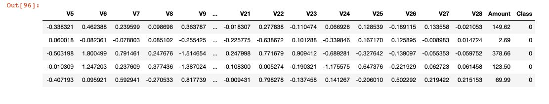
It contains only numerical input variables which are the result of a PCA transformation. Unfortunately, due to confidentiality issues, the original features are not provided. Features V1, V2, … V28 are the principal components obtained with PCA, the only features which have not been transformed with PCA are ‘Time’ and ‘Amount’. Feature ‘Time’ contains the seconds elapsed between each transaction and the first transaction in the dataset. The feature ‘Amount’ is the transaction Amount, this feature can be used for example-dependant cost-sensitive learning. Feature ‘Class’ is the response variable and it takes value 1 in case of fraud and 0 otherwise.
### General
import numpy as np
import pandas as pd
import matplotlib.pyplot as plt
df = pd.read_csv('creditcard.csv')
df.head()
If you explore the data, you’ll notice that only 0.17% of the transactions are fraudulent. We’ll use the F1-Score metric, a harmonic mean between the precision and the recall.
To understand the nature of the fraudulant transactions, simply plot the following graph :
plt.figure(figsize=(12,8))
plt.scatter(df[df.Class == 0].Time, df[df.Class == 0].Amount, c='green', alpha=0.4, label="Not Fraud")
plt.scatter(df[df.Class == 1].Time, df[df.Class == 1].Amount, c='red', label="Fraud")
plt.title("Amount of the transaction over time")
plt.legend()
plt.show()
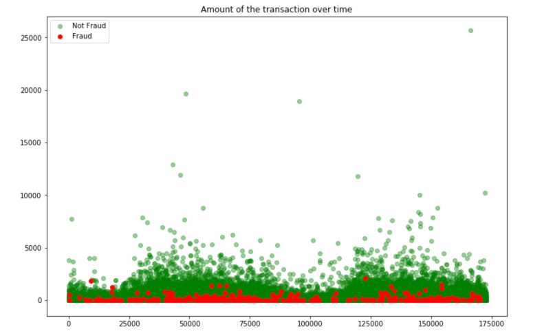
Fraudulent transactions have a limited amount. We can guess that these transactions must remain “unseen” and not attracting too much attention.
HyperOpt
Import the HyperOpt packages and functions :
### HyperOpt Parameter Tuning
from hyperopt import tpe
from hyperopt import STATUS_OK
from hyperopt import Trials
from hyperopt import hp
from hyperopt import fmin
In this example, we will try to optimize a simple Logistic Regression. Define the maximum number of evaluations and the maximum number of folds :
N_FOLDS = 10
MAX_EVALS = 50
We start by defining an objective function, i.e the function to minimize. Here, we want to maximize the cross validation F1 Score, and therefore minimize 1 - this score.
def objective(params, n_folds = N_FOLDS):
    """Objective function for Logistic Regression Hyperparameter Tuning"""

    # Perform n_fold cross validation with hyperparameters
    # Use early stopping and evaluate based on ROC AUC

    clf = LogisticRegression(**params,random_state=0,verbose =0)
    scores = cross_val_score(clf, X, y, cv=5, scoring='f1_macro')

    # Extract the best score
    best_score = max(scores)

    # Loss must be minimized
    loss = 1 - best_score

    # Dictionary with information for evaluation
    return {'loss': loss, 'params': params, 'status': STATUS_OK}
Then, we define the space, i.e the range of all parameters we want to tune :
space = {
    'class_weight': hp.choice('class_weight', [None, class_weight]),
    'warm_start' : hp.choice('warm_start', [True, False]),
    'fit_intercept' : hp.choice('fit_intercept', [True, False]),
    'tol' : hp.uniform('tol', 0.00001, 0.0001),
    'C' : hp.uniform('C', 0.05, 3),
    'solver' : hp.choice('solver', ['newton-cg', 'lbfgs', 'liblinear', 'sag', 'saga']),
    'max_iter' : hp.choice('max_iter', range(5,1000))
}
We are now ready to run the optimization :
# Algorithm
tpe_algorithm = tpe.suggest

# Trials object to track progress
bayes_trials = Trials()

# Optimize
best = fmin(fn = objective, space = space, algo = tpe.suggest, max_evals = MAX_EVALS, trials = bayes_trials)
You’ll see the progress in a similar way :
2%|▏ | 1/50 [00:31<25:57, 31.78s/it, best loss: 0.4574993225009176]
The variable best contains the model with the best parameters. Now, we simply copy those parameters, define a model :
# Optimal model
clf = LogisticRegression(
    C= 2.959250240545696,
    fit_intercept= True,
    max_iter= 245,
    solver= 'newton-cg',
    tol= 2.335533830757049e-05,
    warm_start= True)
And fit-predict this model :
# Fit-Predict
clf.fit(X_train, y_train)
y_pred =clf.predict(X_test)
f1_score(y_pred, y_test)
0.7356321839080459
Conclusion : I hope this article on Bayesian Hyperparameter Optimization was clear. Don’t hesitate to drop a comment if you have a question/remark.
Sources :