
So far, we covered Markov Chains. Now, we’ll dive into more complex models: Hidden Markov Models.
Hidden Markov Models (HMM) are widely used for :
- speech recognition
- writing recognition
- object or face detection
- part-of-speech tagging and other NLP tasks…
I recommend checking the introduction made by Luis Serrano on HMM on YouTube
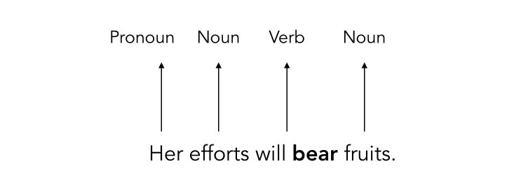
We will be focusing on Part-of-Speech (PoS) tagging. Part-of-speech tagging is the process by which we can tag a given word as being a noun, pronoun, verb, adverb…
PoS can, for example, be used for Text to Speech conversion or Word sense disambiguation.
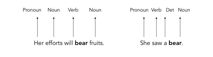
In this specific case, the same word bear has completely different meanings, and the corresponding PoS is therefore different.
Let’s consider the following scenario. In your office, 2 colleagues talk a lot. You know they either talk about Work or Holidays. Since they look cool, you’d like to join them. But you’re too far to understand the whole conversation, and you only get some words of the sentence
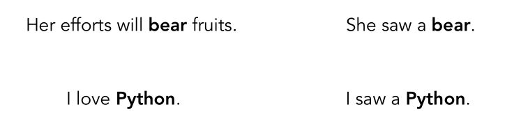
Before joining the conversation, in order not to sound too weird, you’d like to guess whether he talks about Work or Holidays. For example, here is the kind of sentence your friends might be pronouncing :
Emission probabilities
You only hear distinctively the words python or bear, and try to guess the context of the sentence. Since your friends are Python developers, when they talk about work, they talk about Python 80% of the time.
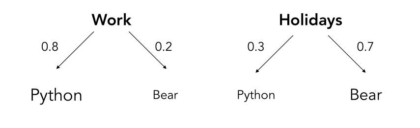
These probabilities are called the Emission probabilities.
Transition probabilities
You listen to their conversations and keep trying to understand the subject every minute. There is some sort of coherence in the conversation of your friends. Indeed, if one hour they talk about work, there is a lower probability that the next minute they talk about holidays.
We can define what we call the Hidden Markov Model for this situation :
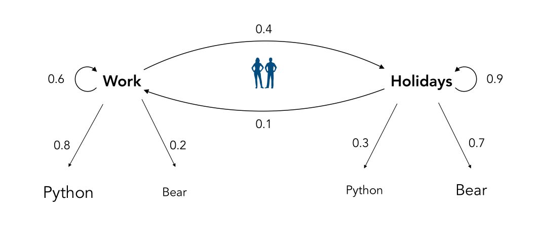
The probabilities to change the topic of the conversation or not are called the transition probabilities.
- The words you understand are called the observations since you observe them. Logic.
- The subject they talk about is called the hidden state since you can’t observe it
Discrete Hidden Markov Models
An HMM \(\lambda\) is a sequence made of a combination of 2 stochastic processes :
- an observed one : \(O = o_1, o_2, ..., o_T\), here the words
- a hidden one : \(q = q_1, q_2, ... q_T\), here the topic of the conversation. This is called the state of the process.
A HMM model is defined by :
- the vector of initial probabilities \(\pi = [ \pi_1, ... \pi_q ]\), where \(\pi_i = P(q_1 = i)\)
- a transition matrix for unobserved sequence \(A\) : \(A = [a_{ij}] = P(q_t = j \mid q_{t-1} = j)\)
- a matrix of the probabilities of the observations \(B = [b_{ki}] = P(o_t = s_k \mid q_t = i)\)
What are the main hypothesis behind HMMs ?
- independence of the observations conditionally to the hidden states : \(P(o_1, ..., o_t, ..., o_T \mid q_1, ..., q_t, ..., q_T, \lambda) = \prod_i P(o_t \mid q_t, \lambda)\)
- the stationary Markov Chain : \(P(q_1, q_2, ..., q_T) = P(q_1) P(q_2 \mid q_1) P(q_3 \mid q_2) ... P(q_T \mid q_{T-1})\)
- Joint probability for a sequence of observations and states : \(P(o_1, o_2, ... o_T, q_1, ..., q_T \mid \lambda) = P(o_1, ..., o_T \mid q_1, ..., q_T, \lambda) P(q_1, ..., q_T)\)
An HMM is a subcase of Bayesian Networks.
How can we find the transition probabilities?
They are based on the observations we have made. We can suppose that after carefully listening, every minute, we manage to understand the topic they were talking about. This does not give us the full information on the topic they are currently talking about though.
You have 15 observations, taken over the last 15 minutes, W denotes Work and H Holidays.
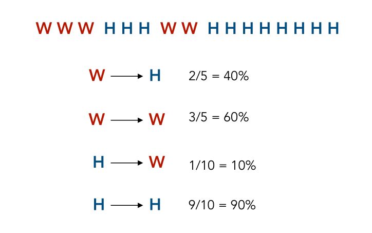
We notice that in 2 cases out of 5, the topic Work lead to the topic Holidays, which explains the transition probability in the graph above.
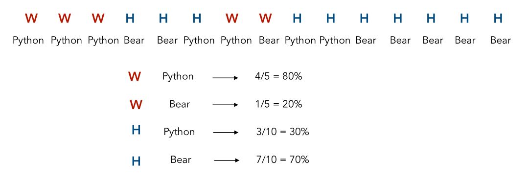
How can we find the emission probabilities?
Well, since we have observations on the topic they were discussing, and we observe the words that were used during the discussion, we can define estimates of the emission probabilities :
What is the probability for each topic at a random minute?
Suppose that you have to grab a coffee, and when you come back, they are still talking. You have no clue what they are talking about! What is at that random moment the probability that they are talking about Work or Holidays?
We can count from the previous observations: 10 times they were talking about Holidays, 5 times about Work. Therefore, it states that we have \(\frac {1} {3}\) chance that they talk about Work, and \(\frac {2} {3}\) chance that they talk about Holidays.
If you hear the word “Python”, what is the probability of each topic?
If you hear the word “Python”, the probability that the topic is Work or Holidays is defined by Bayes Theorem!
\[P(Work \mid Python) = \frac { P(Python \mid Work) P(Work) } {P(Python)}\]We can replace the probabilities :
\[P(Work \mid Python) = \frac { 0.8 \times \frac {1} {3} } { 0.3 \times \frac {2} {3} + 0.8 \times \frac {1} {3}}\]Which heads to 57%.
If you hear a sequence of words, what is the probability of each topic?
Let’s start with 2 observations in a row. Let’s suppose that we hear the words “Python” and “Bear” in a row. What are the possible combinations?
- Python was linked to Work, Bear was linked to work
- Python was linked to Holidays, Bear was linked to work
- Python was linked to Holidays, Bear was linked to Holidays
- Python was linked to Work, Bear was linked to Holidays
These scenarios can be summarized this way :
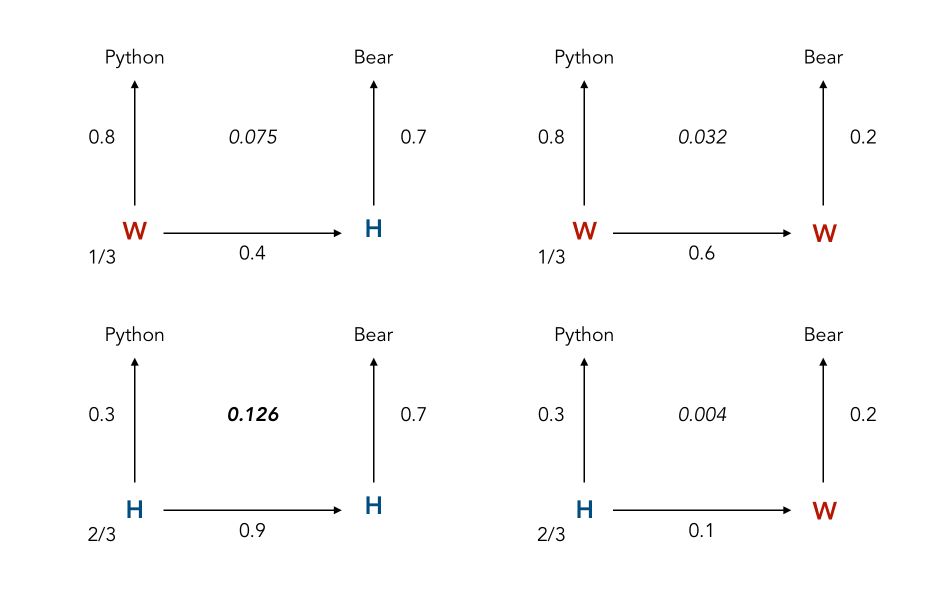
Therefore, the most likely hidden states are Holidays and Holidays. What if you hear more than 2 words? Let’s say 50? It becomes challenging to compute all the possible paths! This is why the Viterbi Algorithm was introduced, to overcome this issue.
Decoding with Viterbi Algorithm
The main idea behind the Viterbi Algorithm is that when we compute the optimal decoding sequence, we don’t keep all the potential paths, but only the path corresponding to the maximum likelihood.
Here’s how it works. We start with a sequence of observed events, say Python, Python, Python, Bear, Bear, Python. This sequence corresponds simply to a sequence of observations : \(P(o_1, o_2, ..., o_T \mid \lambda_m)\).
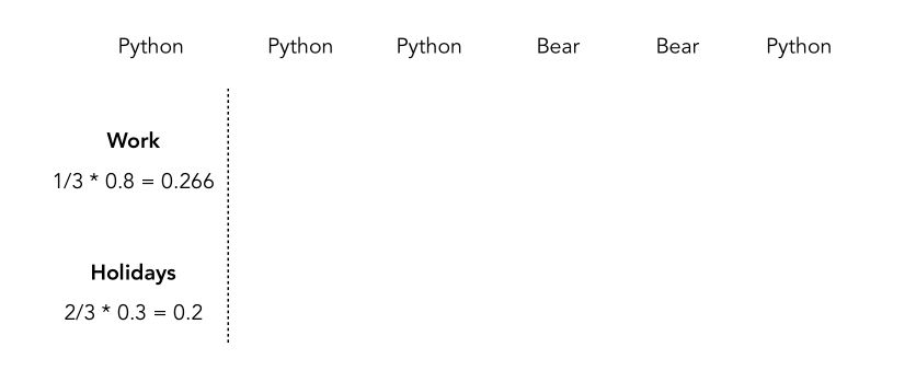
For the first observation, the probability that the subject is Work given that we observe Python is the probability that it is Work times the probability that it is Python given that it is Work.
The most likely sequence of states simply corresponds to : \(\hat{m} = argmax_m P(o_1, o_2, ..., o_T \mid \lambda_m)\)
We can then move on to the next day. Here’s what will happen :
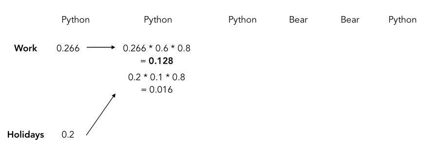
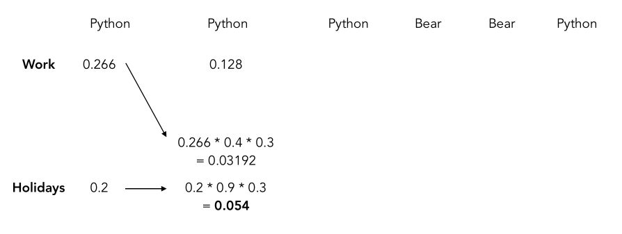
For each position, we compute the probability using the fact that the previous topic was either Work or Holidays, and for each case, we only keep the maximum since we aim to find the maximum likelihood. Therefore, the next step is to estimate the same thing for the Holidays topic and keep the maximum between the 2 paths.
If you decode the whole sequence, you should get something similar to this (I’ve rounded the values, so you might get slightly different results) :
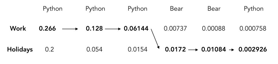
The most likely sequence when we observe Python, Python, Python, Bear, Bear, Python is, therefore Work, Work, Work, Holidays, Holidays, Holidays.
If you finally go talk to your colleagues after such a long stalking time, you should expect them to be talking about holidays :)
Let’s go a little deeper in the Viterbi Algorithm and formulate it properly.
The joint probability of the best sequence of potential states ending in-state \(i\) at time \(t\) and corresponding to observations \(o_1, ..., o_T\) is denoted by \(\delta_T(i)\). This is one of the potential paths described above.
\[\delta_T(i) = max_{q_1, ..., q_{t+1}} P(q_1, ... q_t = i, o_1, ..., o_t, o_{t+1} \mid \lambda)\]By recursion, it can be shown that :
\[\delta_{t+1}(j) = b_j(o_{t+1}) max_i a_{ij} \delta_t{i}\]Where \(b_j\) denotes a probability of the matrix of observations \(B\) and \(a_{ij}\) denotes a value of the transition matrix for unobserved sequence. Those parameters are estimated from the sequence of observations and states available. The \(\delta\) is simply the maximum we take at each step when moving forward.
I won’t go into further details here. You should simply remember that there are 2 ways to solve Viterbi, forward (as we have seen) and backward.
When we only observe partially the sequence and face incomplete data, the EM algorithm is used.
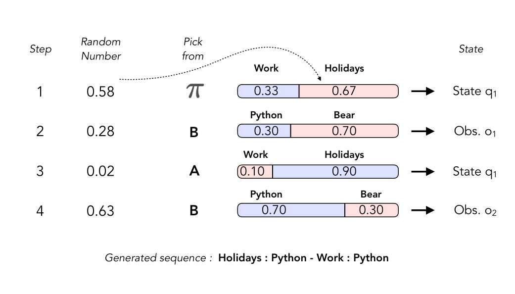
Generating a sequence
As we have seen with Markov Chains, we can generate sequences with HMMs. In order to do so, we need to :
- generate first the hidden state \(q_1\) then \(o_1\), e.g Work then Python
- then generate the transition \(q_1\) to \(q_2\)
- then from \(q_2\), generate \(o_2\)
How does the process work? As stated above, this is now a 2 step process, where we first generate the state, then the observation.
Conclusion : I hope this was clear enough! HMMs are interesting topics, so don’t hesitate to drop a comment!