In this series of articles, we’ll focus on Markov Models, where an when they should be used, and extensions such as Hidden Markov Models.

We’ll cover into further details when to use Markov Models. For the moment, one should remember that Markov Models, and especially Hidden Markov Models (HMM) are used for :

speech recognition
writing recognition
object or face detection
and several NLP tasks …

I. Stochastic model

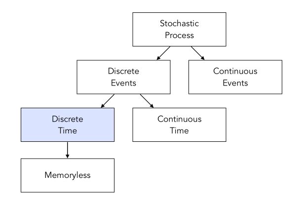
Let’s start by defining what a stochastic model is. It is essentially a discrete-time process \(q_1, q_2, ...\) indexed at times \(1, 2, ...\) whose “states” are observed. The states simply correspond to the actual values of the process, usually defined by a finite space: \(S = 1, ... Q\).

The process starts at an initial state \(q_1\). Then, according to transition probabilities, we move between the states. We can compute the probability of a sequence of states using Bayes Rule :

\[P(q_1, q_2, ... q_T) = P(q_T \mid q_1, q_2, ... q_{T-1}) \times P(q_1, q_2, ... q_{T-1} )\] \[= P(q_T \mid q_1, q_2, ... q_{T-1}) \times P(q_{T-1} \mid q_1, q_2, ... q_{T-2}) \times P(q_1, q_2, ... q_{T-2} ) = ...\] \[= P(q_1) P(q_2 \mid q_1) P(q_3 \mid q_1, q_2) ... P(q_T \mid q_1, q_2, ... q_{T-1})\]

To characterize the model, we need :

the initial probability \(P(q_1)\)
all the transition probabilities

As you might guess, this is complex to achieve since we need to know a lot of parameters.

II. Discrete Time Markov Chain Models (DTMC)

What is a Markov Chain?

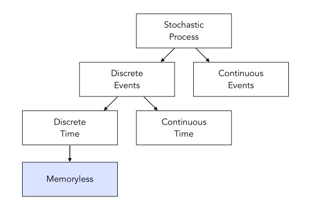
Discrete Time Markov Chain (DTMC) are time and event discrete stochastic process. Markov Chains rely on the Markov Property that there is a limited dependence within the process :

\(P(q_t \mid q_1, ..., q_{t-1}) = P(q_t \mid q_{t-k}, ..., q_{t-1})\) where \(k = 1\) or \(2\).

When \(k = 1\), \(P(q_t \mid q_1, ..., q_{t-1}) = P(q_t \mid q_{t-1})\)

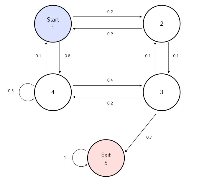
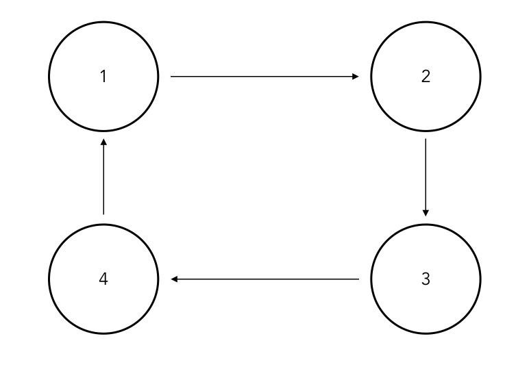
\[P(q_1, q_2, ..., q_T) = P(q_1) P(q_2 \mid q_1) ... P(q_T \mid q_{T-1})\]

Let’s illustrate this! Consider a simple maze in which a mouse is trapped. We will denote \(q_t\) the position of the maze in which the mouse stands after \(t\) steps. We will assume that the mouse does not have a memory of the steps it took within the maze. It simply goes to the position randomly, following the probability written next to each move.

The states here could represent may things, including an NLP project, e.g 1 = Noun, 2 = Verb, 3 = Adjective… and we would be interested in the probabilities have a verb after a noun for example.

Transition probabilities and matrix

A Discrete Time Markov chain is said to be homogeneous if its transition probabilities do not depend on the the \(t\) :

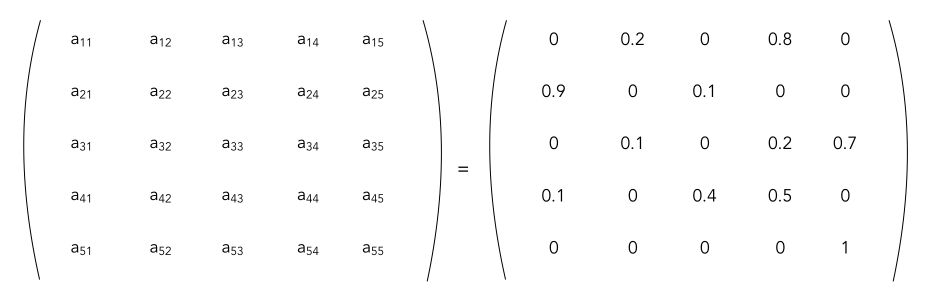
\[P(q_t = j \mid q_{t-1} = i) = P(q_{t+k} = j \mid q_{t+k-1} = i) = a_{ij}\]

We can summarize the process is a transition matrix denoted \(A = [a_{ij}], i \in 1...Q, j \in 1...Q\). A transition matrix is stochastic if :

all entries are non-negative
each line sums to 1

In our example, the transition matrix would be :

Note that if \(A\) is stochastic, then \(A^n\) is stochastic.

States

There are several ways to describe a state. Let \(p_{ii}\) be the probability of returning to state \(i\) after leaving \(i\) :

a state \(i\) is transient if \(p_{ii} < 1\)
a state \(i\) is recurrent if \(p_{ii} = 1\)
a state \(i\) is absorbing if \(a_{ii} = 1\)

Therefore, a state is positive recurrent if the average time before return to this same state denoted \(T_{ii}\) is finite.

A DTMC is irreducible if a state \(j\) can be reached in a finite number of steps from any other state \(i\). An irreducible DTMC is, in fact, a strongly connected graph.

A state in a discrete-time Markov chain is periodic if the chain can return to the state only at multiples of some integer larger than 1.

For example :

Otherwise, it is called aperiodic. A state with a self-loop, i.e \(a_{ii}\) is always aperiodic.

Sojourn time

Let \(T_i\) be the time spent in state \(i\) before jumping to other states.

Then, \(T_i\) follows a geometric distribution :

\[P(T_i = n) = {a_{ii}}^{n-1}(1-a_{ii})\]

The expected average time spent is \(E(T) = \frac {1}{a_{ii}}\)

m-step transition

The probability of going from \(i\) to \(j\) in \(m\) steps is denoted by :

\[{a_{ij}}^{(m)} = P(X_{n+m} = j \mid X_n = i) = P(X_m = j \mid X_0 = i)\]

We can see \({a_{22}}^(4)\) as the probability for the mouse to still be in position 2 at time \(t = 4\). Therefore, the probability of going from \(i\) to \(j\) in exactly \(n\) steps is given by \({f_{ij}}^(n)\) where :

\[f_{ij} = a_{ij} + \sum_{k≠jj} a_{ik} f_{kj}\]

Probability distribution of states

Let \(\pi_i(n)\) be the probability of being in state \(i\) at time \(n\) : \(\pi_i(n) = P(X_n = i)\).

Then, \(\pi(n) = [ \pi_1(n), \pi_2(n), ...]\) is the vector of probability distribution which depends on :

the initial transition matrix A
the initial distribution \(\pi(0)\)

Notice that : \(\pi(n+1) = \pi(n) A\) and recursively : \(\pi(n) = \pi(0) A^n\)

For an irreducible / aperiodic DTMC, the distribution \(\pi(n)\) converges to a limit vector \(\pi\) which is independent of \(\pi(0)\) and is the unique solution of :

\[\pi = \pi P\]

And :

\[\sum_i \pi_i = 1\]

\(\pi_i\) is also called stationary probabilities, steady-state or equilibrium distribution.

Generating a sequence

When we want to generate a sequence, we start from an initial state \(q_1 = 1\) for example. The general idea is that :

we pick a random number to know which state we should start from
then, pick a random number to know which state we move to

It can be illustrated this way. Suppose we are given the following model :

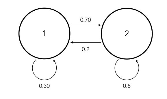
This corresponds to the following matrix \(A\). We are also given the initial vector of probabilities :

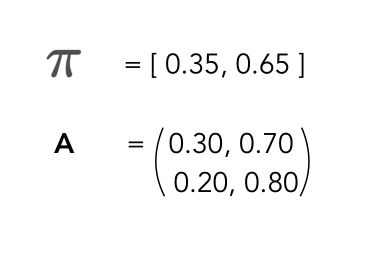
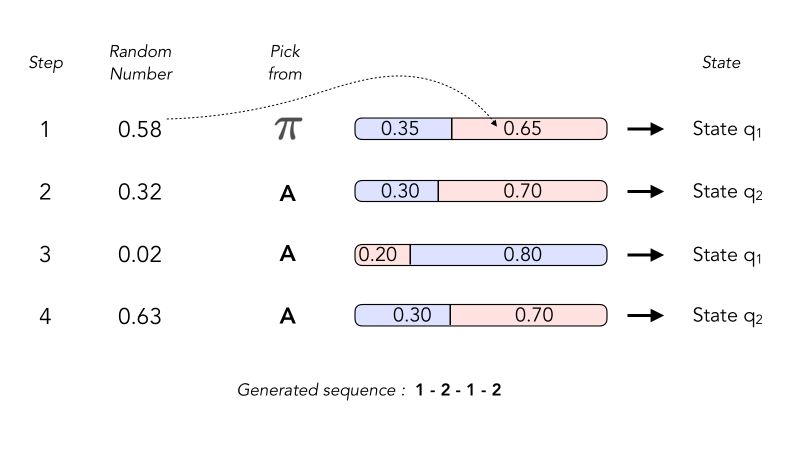
The generator works as follows, by drawing successively random number of identifying which transition is referred to.

III. Let’s code!

Alright, enough theory. We’ll now implement our own Markov Chain in Python.

To do so, download this file (bigramenglish.txt) and this file (bigramfrench.txt).

Those two files are transition matrices for both English and French language, between each letter. They contain transition probabilities between each letter, and we will try to generate words in both languages!

import numpy as np
import matplotlib.pyplot as plt

bi_eng = np.loadtxt('bigramenglish.txt')
bi_fr = np.loadtxt('bigramfrench.txt')

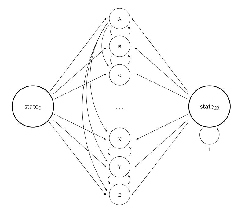
The matrices have size 28 * 28. Why 28?

The first state is the initial state from which we start, not a letter
The 26 next states correspond to a given letter
The final state corresponds to the end of the word

Therefore, the probabilities in the first line correspond to the transition probability from the beginning of the word to the next letter.

Here is a partial schema of the Markov Chain, in which I have represented some of the connexions :

To be able to interpret what is going on, we define a dictionary with the correspondance between the index and the letter :

dic={1 : ' ', 
: 'a', 
: 'b', 
'c', 
: 'd', 
: 'e', 
'f', 
: 'g', 
: 'h', 
'i', 
'j', 
: 'k', 
: 'l', 
'm', 
: 'n', 
: 'o', 
'p', 
: 'q', 
: 'r' , 
's', 
: 't', 
: 'u', 
'v', 
: 'w', 
: 'x' , 
'y', 
: 'z', 
: ' ' }

Generate a word

We will aim to generate a sequence of words. Using what we just covered previously, we can define a function that creates the new state starting from a given state :

def next_state(dic, bi_gram, state) :
    # Generate random threshold
    x = np.random.random()
    # Select the line that corresponds to the state
    line = bi_gram[state-1]
    
    # Find position in which the threshold falls
    thr = np.where(np.cumsum(line)>x)[0][0]+1
    return thr

To understand what this is exactly doing, let’s plot the cumulative distribution and the random threshold :

plt.figure(figsize=(12,8))
plt.plot(np.cumsum(bi_eng[2]))
plt.title("Cumulative Distribution function")
plt.axvline(np.random.random()*28, c='red')
plt.show()

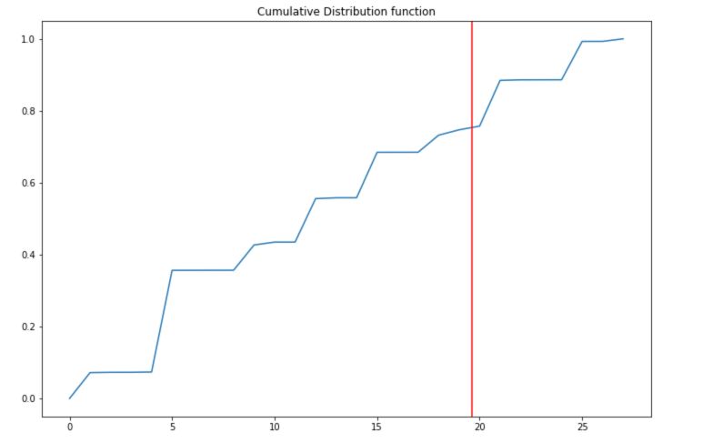
The cumulative function and the threshold allow us to pick a letter starting from a given state. Now, let’s generate a sequence from scratch!

def genere_state_seq(dic, bi_gram) :
    # Start from state 1
    state = 1
    seq = []
    
    # While not reached final state
    while state != 28 :
        # Compute the new state and append
        state = next_state(dic, bi_gram, state)
        seq.append(dic[state])
    return ''.join(seq)

Now, let’s look at some of the words it can generate in english :

for i in range(50) :
    print(genere_state_seq(dic, bi_eng))

Most of the words generated will not mean anything, but be grammatically close to English. You might encounter real words such as the or play.

Generate a sentence

The aim is now to generate a sequence of words to make an actual sentence. We need to modify a bit the transition function :

the end of the sentence will be denoted by .
the end of the word should not be an absorbing state anymore and should either send to the end of the sentence, say with a probability of 10%, or send back to the beginning of the sentence with a probability of 90%.

The next dictionnary will be the following :

dic_2 ={1 : ' ', 
: 'a', 
: 'b', 
'c', 
: 'd', 
: 'e', 
'f', 
: 'g',    
: 'h', 
'i', 
'j', 
: 'k', 
: 'l', 
'm', 
: 'n', 
: 'o', 
'p', 
: 'q', 
: 'r' , 
's', 
: 't', 
: 'u', 
'v', 
: 'w', 
: 'x' , 
'y', 
: 'z', 
: '',
: '.'}

We modify the transition function according to the rules defined above. We need to append a new line and a new column so that the matrix now has a dimension 29*29.

def modify_mat_dic(bi_eng) :

    # Append new column
    new_col = (np.zeros(28)).T
    bi_eng = np.vstack( (bi_eng, new_col) )

    # Append new line
    new_line = np.zeros(29).reshape(-1,1)
    bi_eng = np.hstack( (bi_eng, new_line) )
    
    # Value on bottom right corner is now 1
    bi_eng[-1,-1] = 1

    # Modify before last line (end of word)
    bi_eng[-2] = np.zeros(29)   
    bi_eng[-2,0] = 0.9 # Back to start
    bi_eng[-2,-1] = 0.1 # End of sentence

    return bi_eng
    
bi_eng_mod = modify_mat_dic(bi_eng)
bi_fr_mod = modify_mat_dic(bi_fr)

Then, we need to modify the function that generates the next state to include the next character :

def genere_state_seq_2(dic, bi_gram) :
    state = 1
    seq = []
    while state != 29 :
        state = next_state(dic, bi_gram, state)
        seq.append(dic[state])
    return ''.join(seq)

And finally generate sentences :

for i in range(20) :
    print(genere_state_seq_2(dic_2, bi_eng_mod))

After a few tries I obtained a sentence with 2 real English words :

hernses the holy.

Language Recognition

Markov Chains can also be used to identify the language of a sequence! Indeed, to find the most “likely” language, all we need to do is to multiply the transition probabilities for a given sequence and identify the highest result.

To try this, we’ll modify our dictionary to have specific characters for the beginning and the end of each word, so that the sequence we’ll send it will have the form: to-+be-+or-+not-+to-+be-. for example.

dic_3 ={1 : '+', 
: 'a', 
: 'b', 
'c', 
: 'd', 
: 'e', 
'f', 
: 'g', 
: 'h', 
'i', 
'j', 
: 'k', 
: 'l', 
'm', 
: 'n', 
: 'o', 
'p', 
: 'q', 
: 'r' , 
's', 
: 't', 
: 'u', 
'v', 
: 'w', 
: 'x' , 
'y', 
: 'z', 
: '-',
: '.'}

Let’s now compute the likelihood of a sequence for each language :

def calc_vraisemblance(dic, bi_eng, bi_fr, seq) :
    # The first letter has index 0
    key_0 = 0
    
    # Initialize transition proba to 1
    trans_eng = 1
    trans_fra = 1

    # For each letter of the sequence
    for letter in seq :
        # Find the key of the dictionnary corresponding
        key_1 = [key for key, val in dic.items() if val == letter][0] - 1
        
        # Transition proba is the value from key_0 to key_1 in Transition matrix
        trans_eng = trans_eng * bi_eng[key_0, key_1]
        trans_fra = trans_fra * bi_fr[key_0, key_1]

        # Update the value of the starting state 
        key_0 = [key for key, val in dic.items() if val == letter][0] - 1

    if trans_eng > trans_fra :
        print("It's English !")
    else :
        print("It's French !")  

    return trans_eng, trans_fra

We can now try our model :)

calc_vraisemblance(dic_3, bi_eng_mod, bi_fr_mod, 'etre-+ou-+ne-+pas-+etre-.')

It's French !
(4.462288711775253e-24, 1.145706887234789e-19)

And on an english sequence :

calc_vraisemblance(dic_3, bi_eng_mod, bi_fr_mod, 'to-+be-+or-+not-+to-+be-.')

It's English !
(8.112892227809415e-20, 5.9602081018686406e-30)

The models we presented here a simplistic but useful to understand deeply what is going on.

Conclusion : I hope this quick introduction to Markov Chains was helpful. Let me know in the comments what sequence of words you have ! :)

Markov Processes

Maël Fabien