
In the previous article, we covered the Gradient Boosting Regression. In this article, we’ll get into the Gradient Boosting Classification.
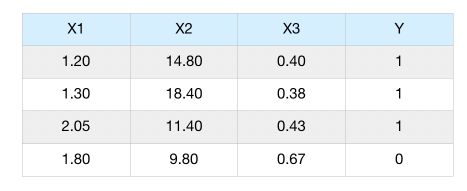
Let’s consider a simple scenario in which we have several features, \(x_1, x_2, x_3, x_4\) and try to predict \(y\), a binary output.
Gradient Boosting Classification steps
Step 1 : Make the first guess
The initial guess of the Gradient Boosting algorithm is to predict the log of the odds of the target \(y\), the equivalent of the average for the logistic regression.
\[odds = log( \frac {P(Y=1)} {P(Y=0)} ) = log( \frac {3} {1} ) = log(3)\]How is this ratio used to make a classification? We apply a softmax transformation!
\[P(Y=1) = \frac {e^{odds}} {1 + e^{odds}} = \frac {3} {4} = 0.75\]If this probability is greater than 0.5, we classify as 1. Else, we classify as 0.
Step 2 : Compute the pseudo-residuals
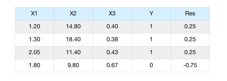
For the variable \(x_1\), we compute the difference between the observations and the prediction we made. This is called the pseudo-residuals.
We have now predicted a value for every sample, the same value for all of them. The next step is to compute the residuals :
Step 3 : Predict the pseudo-residuals
As previously, we use the features 1 to 3 to predict the residuals. Suppose that we build the classification tree to predict the output value of the tree :
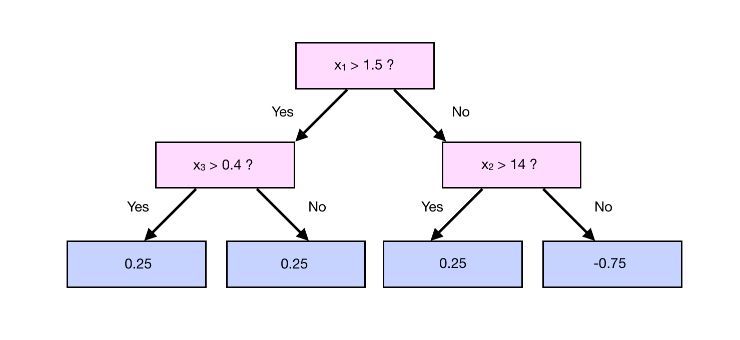
In that case, we cannot use the output of a leaf (or the average output if we have more observations) as the predicted value, since we applied a transformation initiative.
We need to apply another transformation :
\[\gamma_{i+1} = \frac { \sum_i Residuals_i } { \sum(\gamma_i \times (1-\gamma_i))}\]For example, take a case in which we have 1 more observation that falls into a leaf :

In that case, the output value of the branch that contains 0.25 and -0.75 is :
\[\frac {0.25 - 0.75} { 0.75 * (1-0.75) + 0.75*(1-0.75)} = -1.33\]Step 4 : Make a prediction and compute the residuals
We can now compute the new prediction :
\[y_{pred} = odds + lr \times y_{res} = log(3) + 0.1 * -1.33 = 0.9656\]We can now convert the new log odds prediction into a probability using the softmax function :
\[P(Y=1) = \frac {e^{0.9656}} {1 + e^{0.9656}} = 0.7242\]The probability diminishes compared to before since we had 1 well classified and 1 incorrectly classified sample in this leaf.
Step 5 : Make a second prediction
Now, we :
- build a second tree
- compute the prediction using this second tree
- compute the residuals according to the prediction
- build the third tree
- …
As before, we compute the prediction using :
\[y_{pred} = odds + lr \times y_{res} + lr \times y_{res_2} + lr \times y_{res_3} + lr \times y_{res_4} + ...\]And classifiy using :
\[P(Y=1) = \frac {e^{y_{pred}}} {1 + e^{y_{pred}}}\]Conclusion : I hope this introduction to Gradient Boosting Classification was helpful. The topic can get much more complex over time, and the implementation is Scikit-learn is much more complex than this. In the next article, we’ll cover the topic of classification.