
In the previous article, I presented AdaBoost, a powerful boosting algorithm which brings some modifications compared to bagging algorithms. In this article, I’ll present the key concepts of Gradient Boosting. Regression and classification are quite different concepts for Gradient Boosting. In this article, we’ll focus on regression.
Gradient Boosting vs. AdaBoost
Gradient Boosting can be compared to AdaBoost, but has a few differences :
- Instead of growing a forest of stumps, we initially predict the average (since it’s regression here) of the y-column and build a decision tree based on that value.
- Like in AdaBoost, the next tree depends on the error of the previous one.
- But unlike AdaBoost, the tree we grow is not only a stump but a real decision tree.
- As in AdaBoost, there is a weight associated with the trees, but the scale factor is applied to all the trees.
Gradient Boosting steps
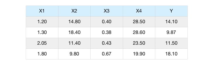
Let’s consider a simple scenario in which we have several features, \(x_1, x_2, x_3, x_4\) and try to predict \(y\).
Step 1 : Make the first guess
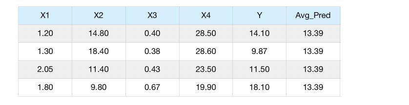
The initial guess of the Gradient Boosting algorithm is to predict the average value of the target \(y\). For example, if our features are the age \(x_1\) and the height \(x_2\) of a person… and we want to predict the weight of the person.
Step 2 : Compute the pseudo-residuals
For the variable \(x_1\), we compute the difference between the observations and the prediction we made. This is called the pseudo-residuals.
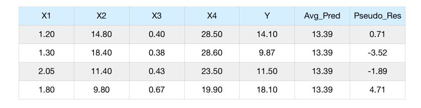
We compute the pseudo-residuals for the first feature \(x_1\).
Step 3 : Predict the pseudo-residuals
Then, we will be using the features \(x_1, x_2,x_3, x_4\) to predict the pseudo-residuals column.
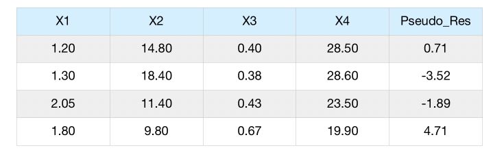
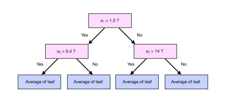
We can now predict the pseudo-residuals using a tree, that typically has 8 to 32 leaves (so larger than a stump). By restricting the number of leaves of the tree we build, we obtain less leaves than residuals. Therefore, the outcome of a given branch of the tree is the average of the columns that lead to this leaf, as in a regression tree.
Step 4 : Make a prediction and compute the residuals
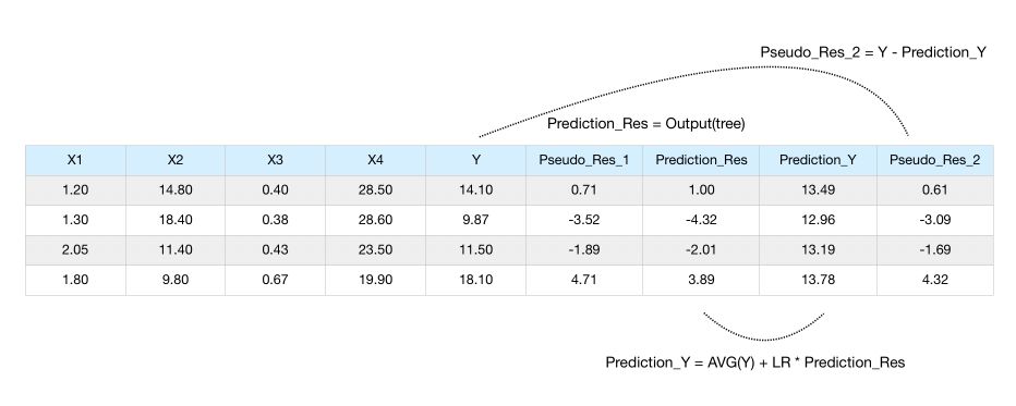
To make a prediction, we say that the average is 13.39. Then, we take our observation, run in through the tree, get the value of the leaf, and add it to 13.39.
If we stop here, we will most probably overfit. Gradient Boost applies a learning rate \(lr\) to scale the contribution from a new tree, by applying a factor between 0 and 1.
\[y_{pred} = \bar{y_{train}} + lr \times res_{pred}\]The idea behind the learning rate is to make a small step in the right direction. This allows an overall lower variance.
Notice how all the residuals got smaller now.
Step 5 : Make a second prediction
Now, we :
- build a second tree
- compute the prediction using this second tree
- compute the residuals according to the prediction
- build the third tree
- …
Let’s just cover how to compute the prediction. We are still using the features \(x_1, x_2, x_3, x_4\) to predict the new residuals Pseudo_Res_2.
We build a tree to estimate those residuals. Once we have this tree (with a limited number of leaves), we are ready to make the new prediction :
\[y_{pred} = \bar{y_{train}} + lr \times res_{pred_1} + lr \times res_{pred_2}\]The prediction is equal to :
- the average value initially computed
- plus LR * the predicted residuals at step 1
- plus LR * the predicted residuals at step 2
Notice how we always apply the same Learning Rate. We are now ready to compute the new residuals, fit the 3rd tree on it, compute the 4th residuals… and so on, until :
- we reach the maximum number of trees specified
- or we don’t learn significantly anymore
Full Pseudo-code
The algorithm can be then described as the following, on a dataset \((x,y)\) with \(x\) the features and \(y\) the targets, with a differentiable loss function \(\cal{L}\):
\(\cal{L} = \frac {1} {2} (Obs - Pred)^2\), called the Squared Residuals. Notice that since the function is differentiable, we have :
\[\frac { \delta } {\delta Pred} \cal{L} = - 1 \times (Obs - Pred)\]Step 1 : Initialize the model with a constant value : \(F_0(x) = argmin_{\gamma} \sum_i \cal{L}(y_i, \gamma)\). We simply want to minimize the sum of the squared residuals (SSR) by choosing the best prediction \(\gamma\).
If we derive the optimal value for \(\gamma\) :
\[\frac { \delta } {\delta \gamma } \sum_i \cal{L}(y_i, \gamma) = -(y_1 - \gamma) + -(y_2 - \gamma) + -(y_3 - \gamma) + ... = 0\] \[\sum_i y_i - n * \gamma = 0\] \[\gamma = \frac{ \sum_i y_i }{n} = \bar{y}\]This is simply the average of the observations. This justifies our previous constant initialization. In other words, we created a leaf that predicts all samples will weight the average of the samples.
Step 2 : For m = 1 to M (the maximum number of trees specified, e.g 100)
- a) Compute the pseudo-residuals for every sample :
This derivative is called the Gradient. The Gradient Boost is named after this.
-
b) Fit a regression tree to the \(r_{im}\) values and create terminal regions \(R_{jm}\) for j = 1, … , \(J_m\), i.e create the leaves of the tree. At that point, we still need to compute the output value of each leaf.
-
c) For each leaf j = 1… \(J_m\), compute the output value that minimized the SSR : \(\gamma_{jm} = argmin_{\gamma} \sum_{x_i \in R_{ij}} \cal{L}(y_i, F_{m-1} + \gamma)\). In other words, we will simply predict the output of all the samples stored in a certain leaf.
-
d) Make a new prediction for each sample by updating, accoridng to a learning rate \(lr \in (0,1)\) : \(F_m(x) = F_{m-1}(x) + lr \times \sum_j \gamma_{jm} I(x \in R_{jm} )\). We compute the new value by summing the previous prediction and all the predictions \(\gamma\) into which our sample falls.
Implement a high-level Gradient Boosting in Python
Since the pseudo-code detailed above might be a bit tricky to understand, I’ve tried to summarize a high-level idea of Gradient Boosting, and we’ll be implementing it in Python.
Step 1 : Initialize the model with a constant value : \(\gamma = \frac{ \sum_i y_i }{n} = \bar{y}\)
This is simply the average of the observations.
Step 2 : For each tree m = 1 to M (the maximum number of trees specified, e.g 100)
- a) Compute the pseudo-residuals for every sample, i.e the true value - the predicted value :
-
b) Fit a regression tree on the residuals, and predict the residuals \(r_t\)
-
c) Update the prediction :
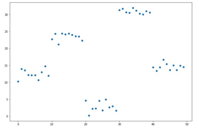
Data generation
We start by generating some data for our regression :
import numpy as np
import pandas as pd
import matplotlib.pyplot as plt

x = np.arange(0,50)
x = pd.DataFrame({'x':x})

y1 = np.random.uniform(10,15,10)
y2 = np.random.uniform(20,25,10)
y3 = np.random.uniform(0,5,10)
y4 = np.random.uniform(30,32,10)
y5 = np.random.uniform(13,17,10)

y = np.concatenate((y1,y2,y3,y4,y5))
y = y[:,None]

plt.figure(figsize=(12,8))
plt.scatter(x,y)
plt.show()
Fit a simple decision tree
To illustrate the limits of decision trees, we can try to fit a simple decision tree with a maximal depth of 1, called a stump.
from sklearn import tree

clf = tree.DecisionTreeRegressor(max_depth=1)
model = clf.fit(x,y)
pred = model.predict(x)

plt.figure(figsize=(12,8))
plt.plot(x, pred, c='red')
plt.scatter(x,y)
plt.show()
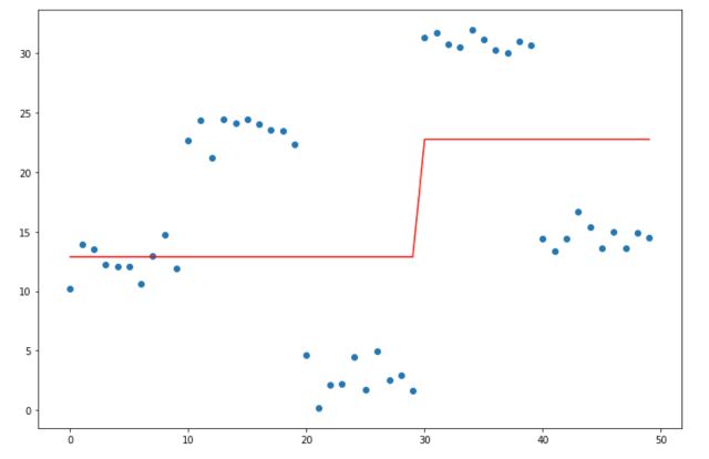
This is the starting point for our estimation. Now, we need to go further and make our model more complex by implementing gradient boosting.
Implement Gradient Boosting
xi = x.copy()
yi = y.copy()

# Initialize error to 0
ei = 0
n = len(yi)

# Initialize predictions with average
predf = np.ones(n) * np.mean(yi)

lr = 0.3

# Iterate according to the number of iterations chosen
for i in range(101):

    # Step 2.a)
    # Fit the decision tree / stump (max_depth = 1) on xi, yi

    clf = tree.DecisionTreeRegressor(max_depth=1)
    model = clf.fit(xi, yi)

    # Use the fitted model to predict yi

    predi = model.predict(xi)

    # Step 2.c)
    # Compute the new prediction (learning rate !)
    # Compute the new residuals,
    # Set the new yi equal to the residuals

    predf = predf + lr * predi
    ei = y.reshape(-1,) - predf
    yi = ei

    # Every 10 iterations, plot the prediction vs the actual data
    if i % 10 == 0 :
        plt.figure(figsize=(12,8))
        plt.plot(x, predf, c='r')
        plt.scatter(x, y)
        plt.title("Iteration " + str(i))
        plt.show()
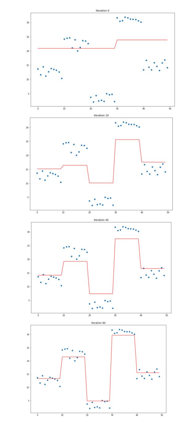
By increasing the learning rate, we tend to overfit. However, if the learning rate is too low, it takes a large number of iterations to even approach the underlying structure of the data.
Conclusion : I hope this introduction to Gradient Boosting was helpful. The topic can get much more complex over time, and the implementation is Scikit-learn is much more complex than this. In the next article, we’ll cover the topic of classification.