In the first part of this two-part series, we explored basic models and data enrichments for our hit song classifier. In this article, we will try to push our model a little more by attempting to improve its performance through better data enrichment and feature engineering. Before we get started, let’s recall the context.

The context

There’s no shortage of articles and papers trying to explain why a song became a hit, and the features hit songs share. Here, we will try to go a bit further and build a hit song classifier. To build such a classifier, we’ll typically need a lot of data enrichment because there is no single source of data that can help with such a large task.

We will use the following sources to help us build the dataset:

Google Trends
Spotify
Billboard
Genius.com

We will consider a song a hit only if it reached the top 10 of the most popular songs of the year. Otherwise, it does not count as a hit.

In part one we used data from the Billboard Year-End Hot100 Singles Chart between 2010 and 2018. We then enriched the data using Spotify’s API. Our model achieved an accuracy of 93% on the test set.

Data Enrichment through Genius.com

Genius.com is a great resource if you are looking for song lyrics. It offers a great API, all of which is packaged in a great library called lyricsgenius. Start by installing the package (instructions can be found on GitHub).

You will have to get a token from Genius.com developer’s website.

Start by importing the package:

import lyricsgenius as genius
api = genius.Genius('YOUR_TOKEN_GOES_HERE')

As before, the API has a powerful search functionality:

def lookup_lyrics(song):
    try :
        return api.search_song(song).lyrics
    except :
        return None

You’ll need to create a column “lyrics” that contains the lyrics of each song. This one might take some time.

df['lyrics'] = df['lookup'].apply(lambda x: lookup_lyrics(x))

Notice how some of the text is not clean and contains \n to denote a new line or has text between brackets to split sections:

def clean_txt(song):
    song = ' '.join(song.split("\n"))
    song = re.sub("[\[].*?[\]]", "", song)
    return song

df['lyrics'] = df['lyrics'].apply(lambda x: clean_txt(x))
df = df.dropna() #Drop song if we don't have lyrics

Some features we could add are:

The length of the lyrics
The number of unique words used
The length of the lyrics without stopwords
The number of unique words used without stopwords

We will use NLTK stop words list in English. However, we should also consider that some of the songs of the Billboard Year-End Hot100 Singles Chart are not English songs.

from nltk.corpus import stopwords 
from nltk.tokenize import word_tokenize 
stop_words = set(stopwords.words('english'))

def len_lyrics(song):
    return len(song.split())

def len_unique_lyrics(song):
    return len(list(set(song.split())))

def rmv_stop_words(song):
    song = [w for w in song.split() if not w in stop_words] 
    return len(song)

def rmv_set_stop_words(song):
    song = [w for w in song.split() if not w in stop_words] 
    return len(list(set(song)))

Next, apply this to the dataset :

df['len_lyrics'] = df['lyrics'].apply(lambda x: len_lyrics(x))
df['len_unique_lyrics'] = df['lyrics'].apply(lambda x: len_unique_lyrics(x))
df['without_stop_words'] = df['lyrics'].apply(lambda x: rmv_stop_words(x))
df['unique_without_stop_words'] = df['lyrics'].apply(lambda x: rmv_set_stop_words(x))

Data exploration

Just like in the first article, some data exploration might bring us additional insights.

How many words are used in the lyrics?

plt.figure(figsize=(12,8))
plt.hist(df[df['len_lyrics']<2000]['len_lyrics'], bins=70) #Not plot outliers
plt.title("Number of words")
plt.show()

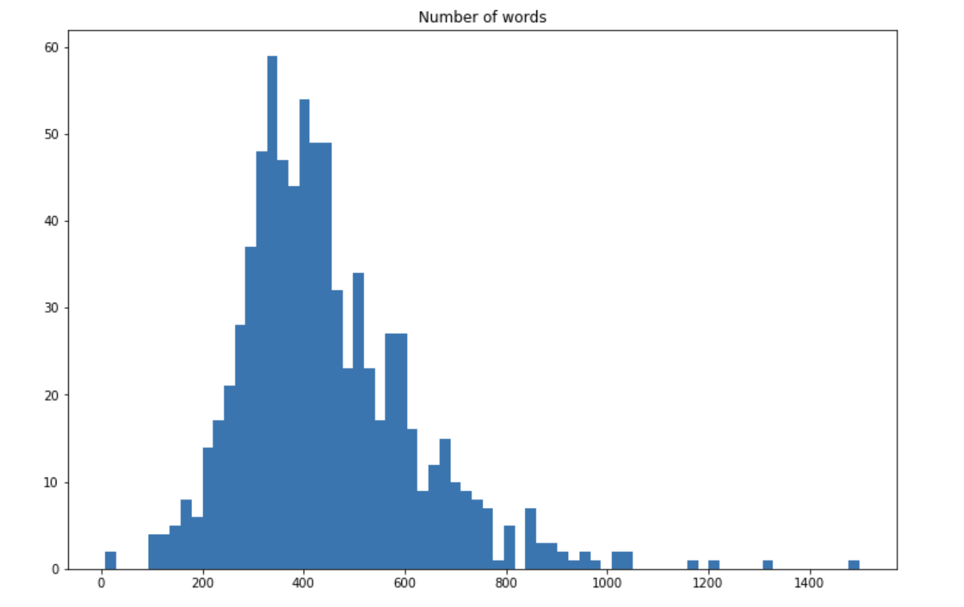
The histogram above does not represent outliers, but a few songs count over 2000 words. On average, there are 467 words in a song and 166 unique words. This can be verified by:

np.mean(df['len_lyrics'])
np.mean(df['len_unique_lyrics'])

The ratio of unique words over total words is 35%. We can also plot the distribution of this ratio:

plt.figure(figsize=(12,8))
plt.hist(df['len_unique_lyrics']/df['len_lyrics'], bins=50)
plt.title("Ratio Unique Words over total words")
plt.show()

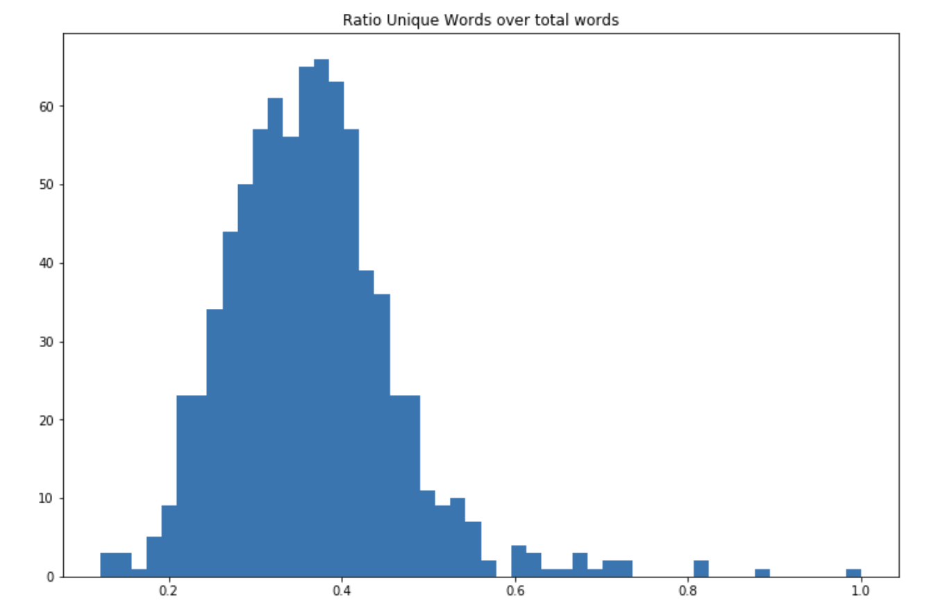
The vast majority of the songs do not exceed 40% of unique words, which reflects the balance that hit songs reach between repetitive lyrics and a diversified vocabulary. The vast majority of To illustrate the diversity of the vocabulary used in the songs, we can compute the ratio of words that are not stop words over all words:

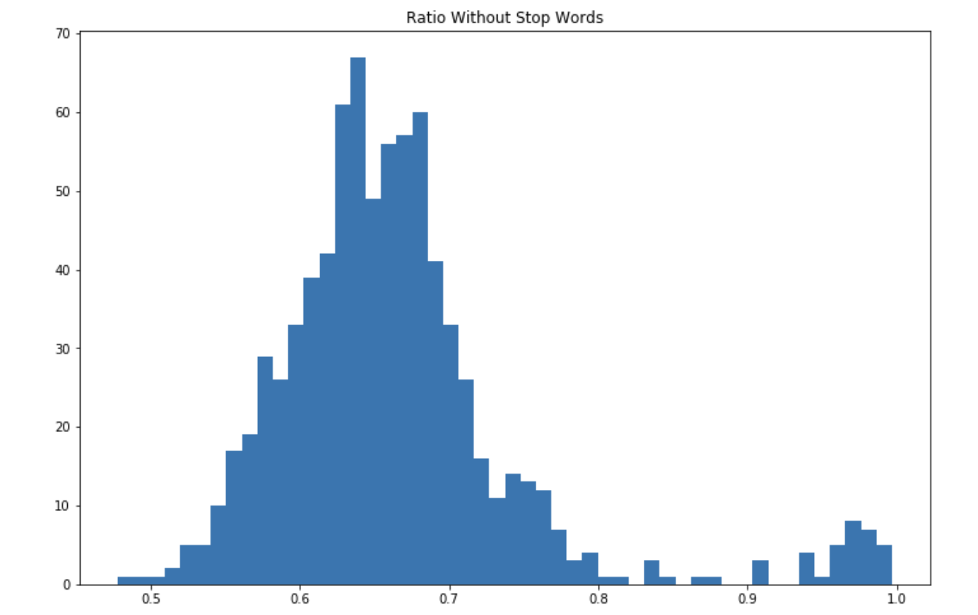
When we remove the stop words, the average ratio is now much higher. A large part of the vocabulary used in those songs seems to be made of stop words. This is it for the count of words. Now, wWhat are the most common words that singers use in their songs?

from wordcloud import WordCloud, STOPWORDS
word_cloud = df['lyrics'].values

str1 = ' '.join(word_cloud)
stopwords = set(STOPWORDS)

wordcloud = WordCloud(stopwords=stopwords, background_color="white").generate(str(str1))

plt.figure(figsize=(15,8))
plt.imshow(wordcloud, interpolation='bilinear')
plt.axis("off")
plt.show()

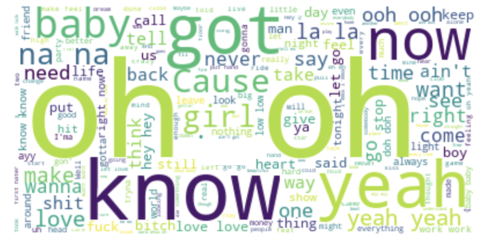
We won’t spend too much time commenting this, but “yeah,” “oh,” and “baby” should definitely be on your hit-song to-do list.

Lyrics sentiment

Should a song be positive? Negative? Neutral? To assess the positiveness of a song and its intensity, we will use Valence Aware Dictionary and sEntiment Reasoner (VADER), a lexicon and rule-based sentiment analysis tool, available on Github. This method relies on lexicons, and has over 7500 words annotated by linguists. This kind of algorithm was used before the rise of Natural Language Processing, but can still be useful in cases like this one where we do not have labeled data or trained models for song sentiment classification.

from vaderSentiment.vaderSentiment import SentimentIntensityAnalyzer
analyzer = SentimentIntensityAnalyzer()

df['sentimentVaderPos'] = df['lyrics'].apply(lambda x: analyzer.polarity_scores(x)['pos'])
df['sentimentVaderNeg'] = df['lyrics'].apply(lambda x: analyzer.polarity_scores(x)['neg'])
df['sentimentVaderComp'] = df['lyrics'].apply(lambda x: analyzer.polarity_scores(x)['compound'])
df['sentimentVaderNeu'] = df['lyrics'].apply(lambda x: analyzer.polarity_scores(x)['neu'])

We can also create a feature that is the difference between the positive and the negative score:

df['Vader'] = df['sentimentVaderPos'] - df['sentimentVaderNeg']

What are the sentiments expressed in the songs?

plt.figure(figsize=(12,8))
plt.hist(df['Vader'], bins=50)
plt.axvline(0, c='r')
plt.title("Average sentiment")
plt.show()

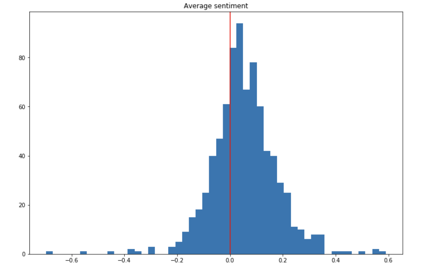
On average, the sentiment is slightly positive. Some songs have strong sentiments attached to them (i.e more than 0.5 in absolute value), but most songs have sentiments that are more controlled. This approach is however limited since it derives the average sentiment of a song by averaging the word sentiments, but does not understand the content and the context.

New model

Now, let’s train a new model and see whether the performance was improved. First, we create the train and test sets and apply oversampling:

X = df.drop(["Artist_Feat", "Artist", "Artist_Feat_Num", "Title", "Hit", "lookup", "release_date", "genres", "lyrics"], axis=1)
y = df["Hit"]

sm = SMOTE(random_state=42)
X_res, y_res = sm.fit_resample(X, y)
X_train, X_test, y_train, y_test = train_test_split(X_res,y_res, test_size=0.2, random_state=42) 

Then, we define the random forest classifier and train the model:

rf=RandomForestClassifier(n_estimators=100)
rf.fit(X_train, y_train)

y_pred = rf.predict(X_test)
accuracy_score(y_pred, y_test)

The accuracy score improved by close to 5% and reaches 98.3%.

What are the most important features in this new model?

importances = rf.feature_importances_
indices = np.argsort(importances)

plt.figure(figsize=(12,8))
plt.title('Feature Importances')
plt.barh(range(len(indices)), importances[indices], align='center')
plt.yticks(range(len(indices)), [X.columns[i] for i in indices])
plt.xlabel('Relative Importance')
plt.show()

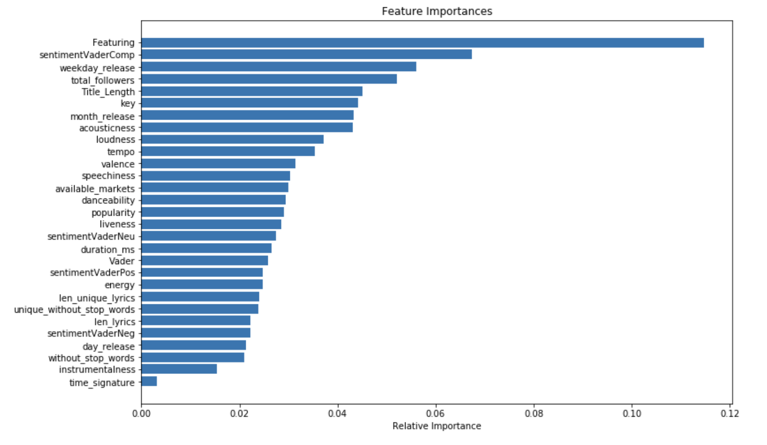
The order of the important features remains the same, but the compound sentiment feature is now one of the most important features.

Making predictions

Prediction function

We can build a predictor that takes the name of the song and the singer as an input, creates the features, and outputs the probability of a song being a hit. Since the algorithm has never been trained on songs from 2019, we can feed it with recent songs and observe the outcome.

Let’s recall the whole pipeline first:

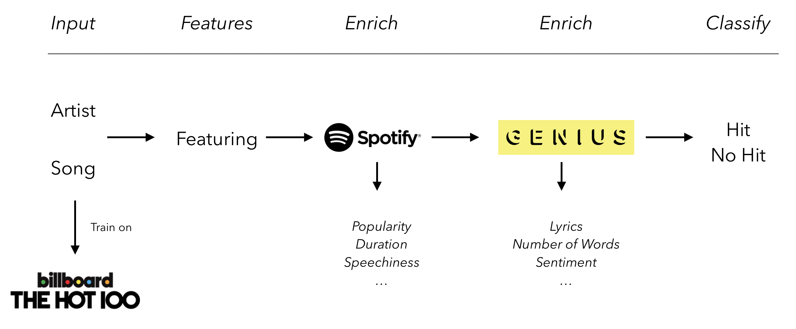
Let’s build this pipeline and try it with “Lover” by Taylor Swift, a song that was recently released when we wrote this article:

def model_prediction(artist, title):
    
    df_pred = pd.DataFrame.from_dict({
        "Artist":[artist], 
        "Title":[title]})
        
    df_pred["Featuring"] = df_pred.apply(lambda row: featuring(row['Artist']), axis=1)
    df_pred["Artist_Feat"] = df_pred.apply(lambda row: featuring_substring(row['Artist']), axis=1)
    df_pred['Title_Length'] = df_pred['Title'].apply(lambda x: num_words(x))
    df_pred['lookup'] = df_pred['Title'] + " " + df_pred["Artist_Feat"]
    df_pred['available_markets'], df_pred['release_date'], df_pred['total_followers'],
    df_pred['genres'], df_pred['popularity'], df_pred['acousticness'], df_pred['danceability'],
    df_pred['duration_ms'], df_pred['energy'], df_pred['instrumentalness'], df_pred['key'],
    df_pred['liveness'], df_pred['loudness'], df_pred['speechiness'], df_pred['tempo'],
    df_pred['time_signature'], df_pred['valence'] = zip(*df_pred['lookup'].map(artist_info))
    df_pred['release_date'] = pd.to_datetime(df_pred['release_date'])
    df_pred['month_release'] = df_pred['release_date'].apply(lambda x: x.month)
    df_pred['day_release'] = df_pred['release_date'].apply(lambda x: x.day)
    df_pred['weekday_release'] = df_pred['release_date'].apply(lambda x: x.weekday())
    df_pred['lookup'] = df_pred['Title'] + " " + df_pred["Artist"]
    df_pred['lyrics'] = df_pred['lookup'].apply(lambda x: lookup_lyrics(x))
    df_pred['lyrics'] = df_pred['lyrics'].apply(lambda x: clean_txt(x))
    df_pred['len_lyrics'] = df_pred['lyrics'].apply(lambda x: len_lyrics(x))
    df_pred['len_unique_lyrics'] = df_pred['lyrics'].apply(lambda x: len_unique_lyrics(x))
    df_pred['without_stop_words'] = df_pred['lyrics'].apply(lambda x: rmv_stop_words(x))
    df_pred['unique_without_stop_words'] = df_pred['lyrics'].apply(lambda x: rmv_set_stop_words(x))
    df_pred['sentimentVaderPos'] = df_pred['lyrics'].apply(lambda x: analyzer.polarity_scores(x)['pos'])
    df_pred['sentimentVaderNeg'] = df_pred['lyrics'].apply(lambda x: analyzer.polarity_scores(x)['neg'])
    df_pred['sentimentVaderComp'] = df_pred['lyrics'].apply(lambda x: analyzer.polarity_scores(x)['compound'])
    df_pred['sentimentVaderNeu'] = df_pred['lyrics'].apply(lambda x: analyzer.polarity_scores(x)['neu'])
    df_pred['Vader'] = df_pred['sentimentVaderPos'] - df_pred['sentimentVaderNeg']

    X = df_pred.drop(["Artist_Feat", "Artist", "Title", "lookup", "release_date", "genres", "lyrics"], axis=1).astype(float)
    y_pred = rf.predict_proba(X)
    
    print("It's a NOT hit with probability : " + str(y_pred[0][0]))
    print("It's a hit with probability : " + str(y_pred[0][1]))
    
    return y_pred

We can create an interactive form the Notebook to ask the user for the name of the artist, title of the song, and output the prediction.

from ipywidgets import widgets, interact

artist = widgets.Text()
title = widgets.Text()

ui = widgets.HBox([artist, title])

def f(artist, title):
    return model_prediction(artist, title)

And in the next cell, type :

interact(f, artist='Taylor Swift', title='Lover')

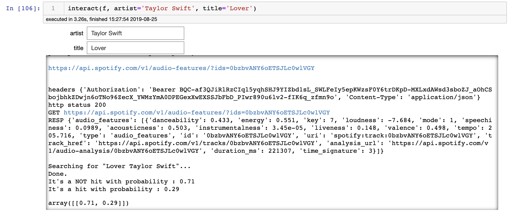
According to our algorithm, there is only a 22% chance that the song “Lover” by Taylor Swift will make it to the top 10 of the most popular songs of 2019. And this is probably the case, since the song “only” peaked at number 10 on Billboard Hot 100 for a few days.

Conclusion

Through this article, we illustrated the importance of external data sources for most data science problems. A good enrichment dataset can boost the performance of your model. Relevant feature engineering can help gain additional performance.

Here is a performance summary of the different steps of our model:

Description	Model	Performance
Data from billboard	Decision Tree	F1-Score : 6.6%
Enrich with Spotify and oversample	Random Forest	Accuracy : 93%
Enrich with Genius	Random Forest	Accuracy : 98%

Sources and resources:

Lyricsgenius

Predicting the next hit song (Part 2)

Maël Fabien