It comes as no surprise that the music industry is tough. When you decide to produce an artist or invest in a marketing campaign for a song, there are many factors to take into account. What if data science could help with this task? What if it could help predict whether a song is going to be a hit or not?

Setting the stage

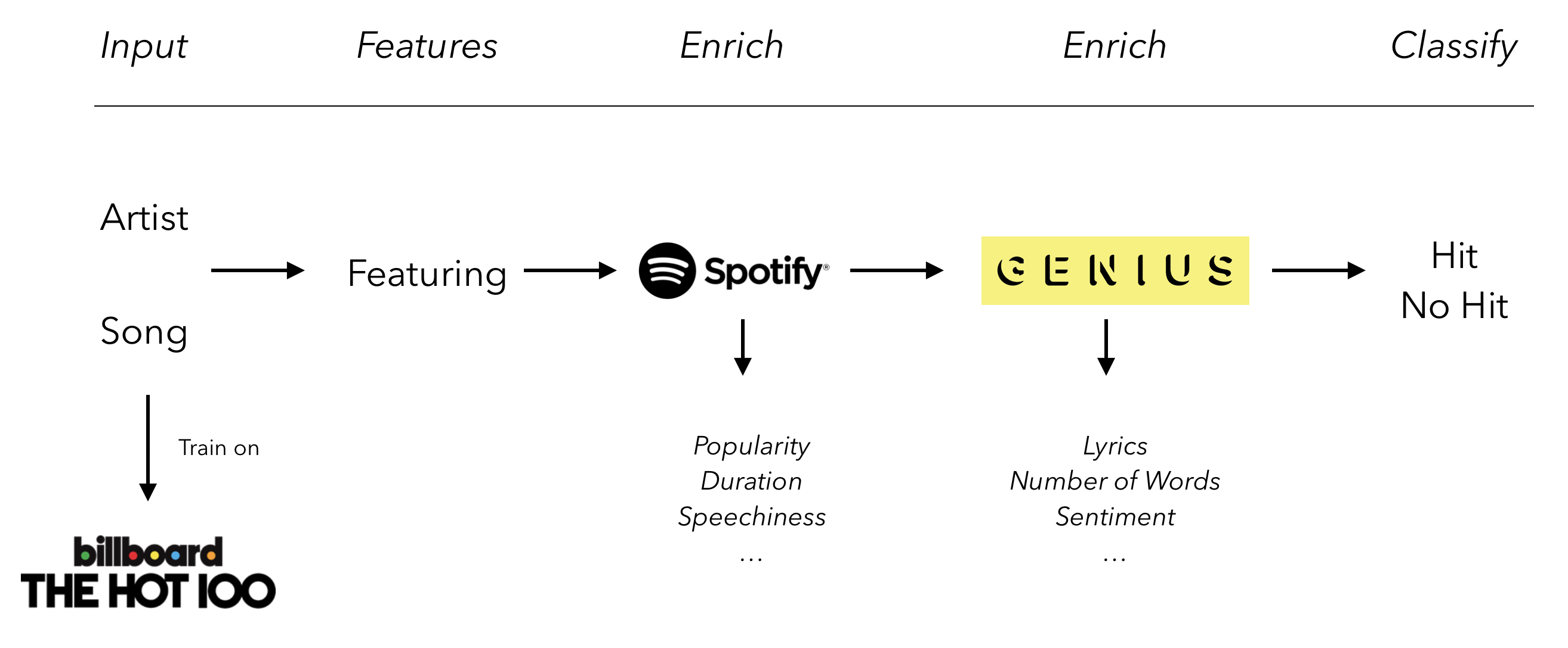
There’s no shortage of articles and papers trying to explain why a song became a hit, and the features hit songs share. Here, we will try to go a bit further and build a hit song classifier. To build such a classifier, we’ll typically need a lot of data enrichment because there is no single source of data that can help with such a large task.

We will use the following sources to help us build the dataset:

Google Trends
Spotify
Billboard
Genius.com

We will consider a song a hit if it reaches the top 10 of the most popular songs of the year. Otherwise, it does not count as a hit.

In this two-part article, we will implement the following pipeline and build our hit song classifier!

Data

Trends

Let’s start by checking the major trends in the music industry using Google Trends.

We will compare the following musical genres:

Pop
Rock
Rap
Country
Jazz

Currently, rap is the leading music genre in the world, having taken over other genres such as rock or pop. A geographical analysis can help us understand which countries listen to what music.

It seems like the US, South Africa and India are strong rap markets, China and Indonesia are strong pop markets, and South America is overall a great rock market.

Top 100

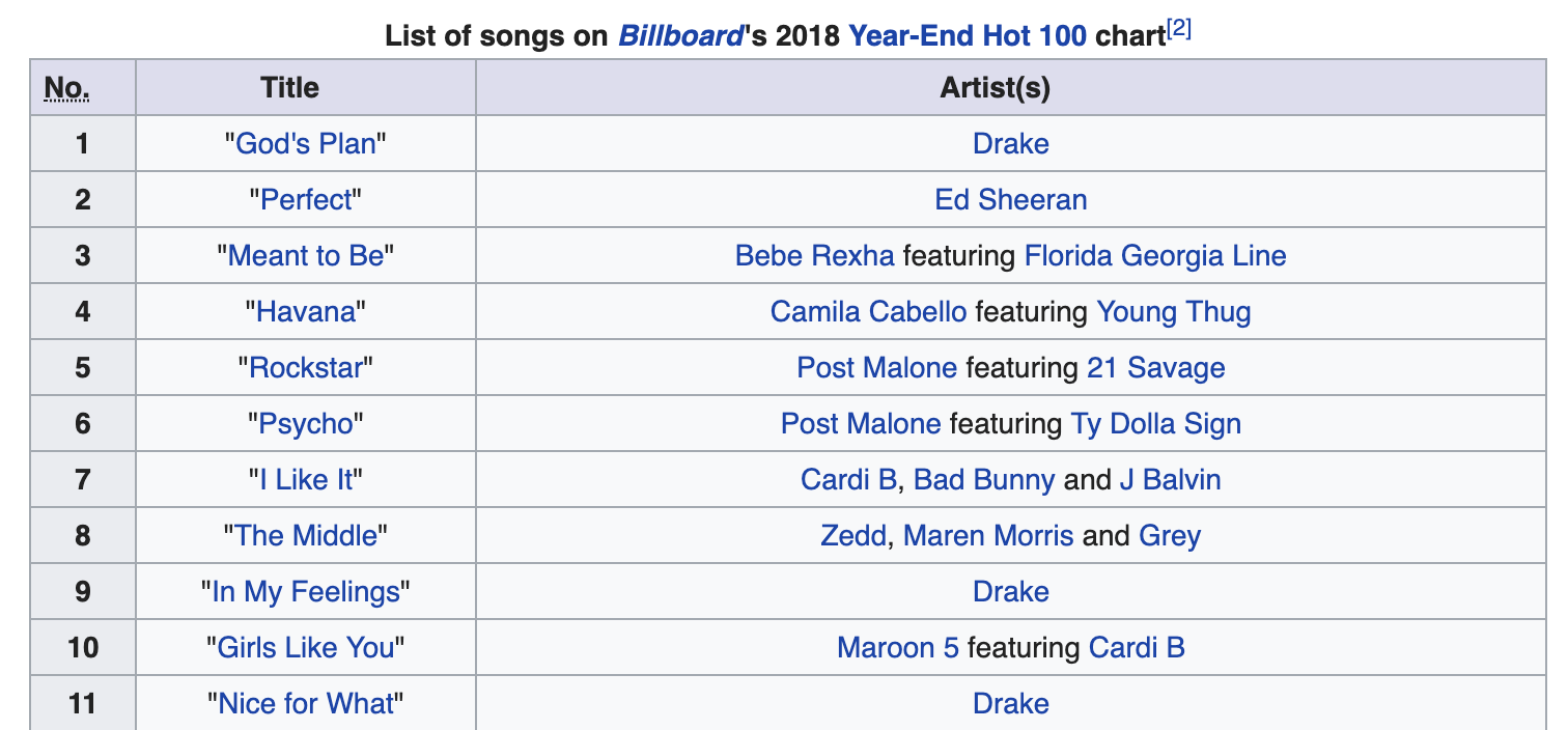
First, we will scrape data from the Billboard Year-End 100 Singles Chart. This will be our main data source. This approach has some limitations since we consider that, for any given song in the training data, it will at least hit the top 100 of the world charts. However, if you are trying to sell an ML-based solution to a music label, knowing whether a song will reach the top 10 of the year or remain at the bottom of the ranking has a huge financial impact.

The year-end chart is calculated using an inverse point system based on the weekly Billboard charts (100 points for a week at number one, 1 point for a week at number 100, etc), for every year since 1946.

Training a classifier using data from 1946 would however make no sense since we need the data to be relevant for the prediction task. Instead, we will focus on data between 2010 and 2018, and make the assumption that the year is not a relevant feature for predicting future hits.

Build the dataset

We first need to retrieve the table from Wikipedia for all the years between 2010 and 2018. Open a notebook, and import the following packages :

import pandas as pd
import matplotlib.pyplot as plt
import re
import requests
from bs4 import BeautifulSoup

We then build a function to handle scraping requests :

def _handle_request(request_result):
    if request_result.status_code == 200:
        html_doc =  request_result.text
        soup = BeautifulSoup(html_doc,"html.parser")
        return soup

The table to scrape is of type table and has the class: wikitable sortable jquery-tablesorter. It can be observed directly from the developer’s console :

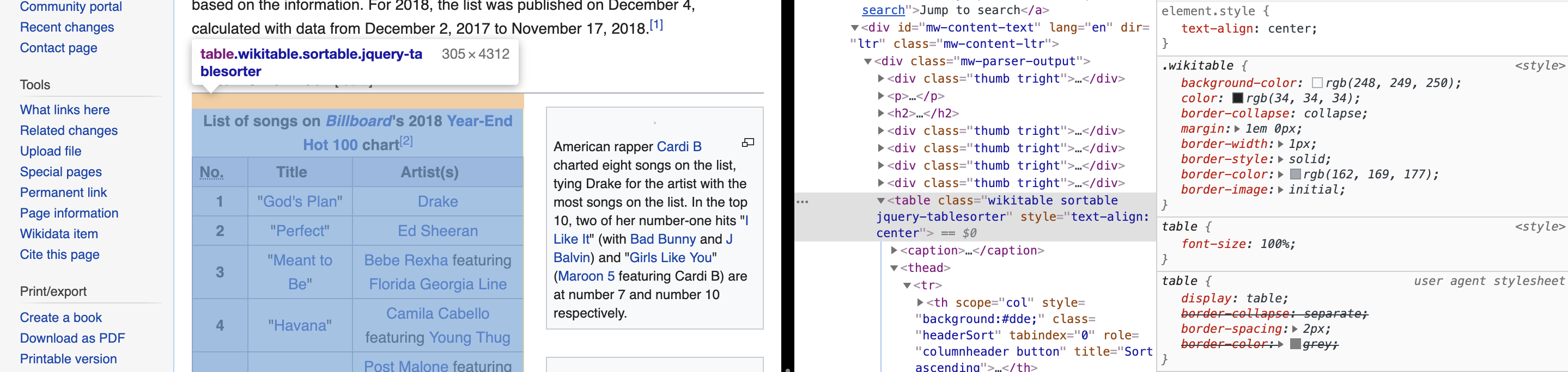
We need to iterate on all the years between 2010 and 2018 :

artist_array = []

for i in range(2010, 2019):

    # Iterate over this link and change year
    website = 'https://en.wikipedia.org/wiki/Billboard_Year-End_Hot_100_singles_of_'+str(i)
    
    # Get the table
    res = requests.get(website)
    specific_class = "wikitable sortable"
    soup = _handle_request(res)
    table = soup.find("table", class_= specific_class)
    
    # Get the body
    table_body = table.find('tbody')
    
    # Get the rows
    rows = table_body.find_all('tr')

    # For each row
    for row in rows:

        try :
            # Find the ranking
            num = row.find_all('th')
            num = [ele.text.strip() for ele in num]
            
            # Assess if the ranking is greater than 1 or not
            if int(num[0]) > 10 :
                num = 0
            else :
                num = 1

            # Find the title and name of artist
            cols = row.find_all('td')
            cols = [ele.text.strip() for ele in cols]
            
            artist_array.append([num, cols[0].replace('"', ''), cols[1]])

        except : 
            pass

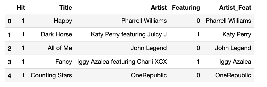
Then, transform this array into a dataframe :

df = pd.DataFrame(artist_array)
df.columns=["Hit", "Title", "Artist"]
df.head(n=10)

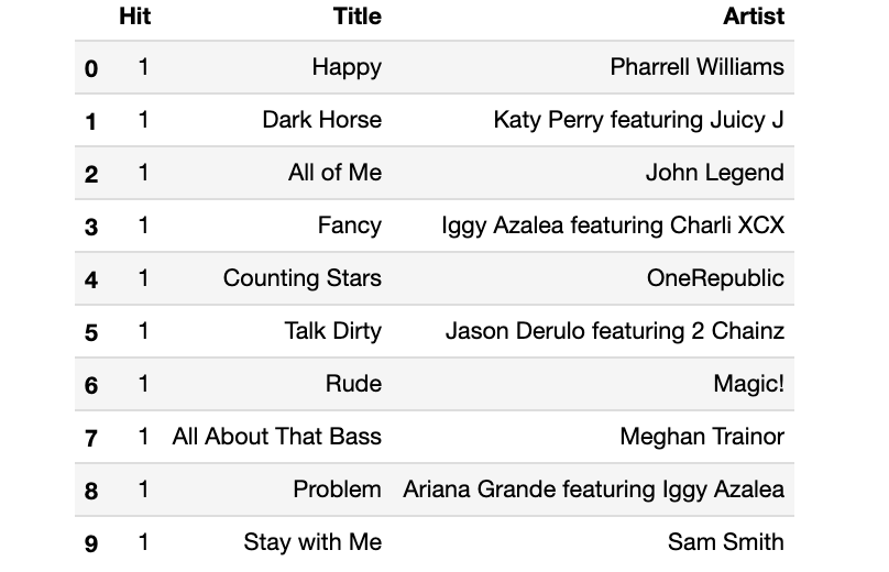
We now have a good amount of data points. Some songs might be on the charts in two different years so next, we want to keep only the first occurrence of a song to avoid having duplicates in the table:

df = df.drop_duplicates(subset=["Title", "Artist"], keep="first")
df.shape

The shape of the data frame is now: (816, 3). Notice that in some cases, the “Artist” column contains “featuring”. We will first create a simple feature where we split the name of the artist column if the word “featuring” is present, and add a feature “featuring” that is equal to “1” if there is a featured artist, and “0” elsewhere.

def featuring(artist):
    if "featuring" in artist :
        return 1
    else :
        return 0

def featuring_substring(artist):
    if "featuring" in artist :
        return artist.split("featuring")[0]
    else :
        return artist

df["Featuring"] = df.apply(lambda row: featuring(row['Artist']), axis=1)
df["Artist_Feat"] = df.apply(lambda row: featuring_substring(row['Artist']), axis=1)

Explore the data

We can quickly explore the data to observe the most popular artists, the number of hits or the number of features. There is, by construction, an imbalance in the number of hits vs. non-hits :

plt.figure(figsize=(10,6))
plt.hist(df["Hit"], bins=3)
plt.title("Non-Hits vs. Hits")
plt.show()

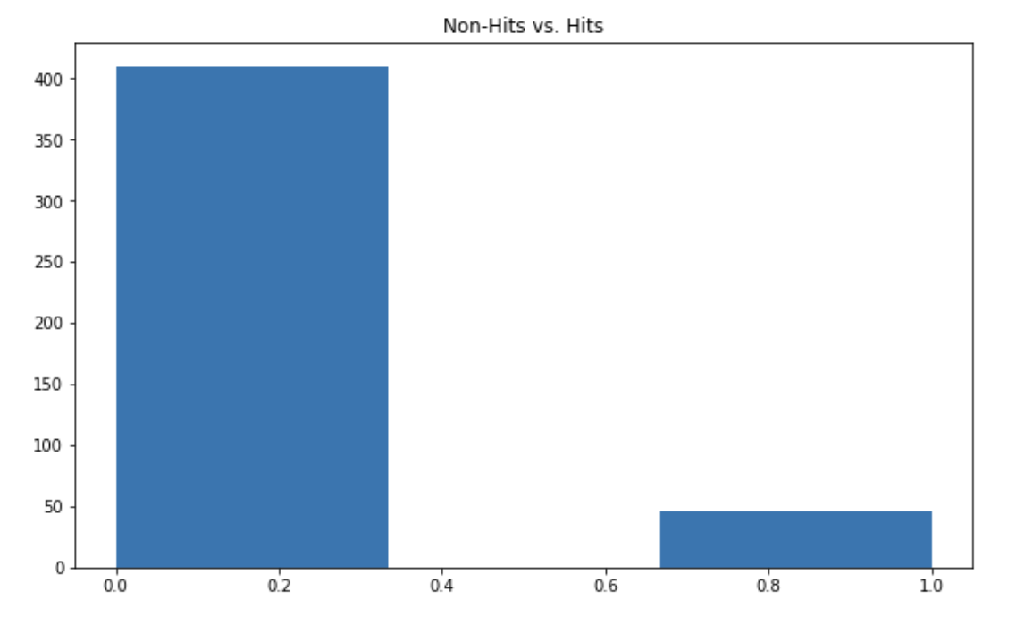
To assess the performance of a model, we will use the F1-score, which handles unbalanced datasets by providing a harmonic average between the precision and the recall.

Is it common for hit songs to feature other artists?

plt.figure(figsize=(10,6))
plt.hist(df["Featuring"], bins=3)
plt.title("No Featuring vs. Featuring")
plt.show()

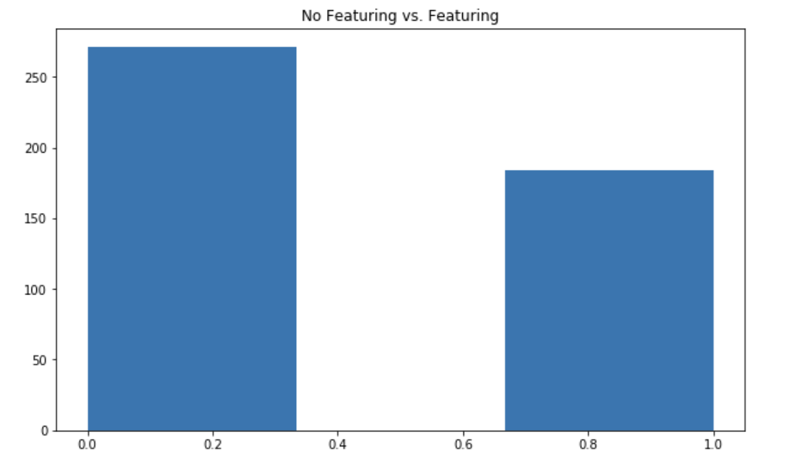
Most hit songs feature other artists! This is an interesting point since in most albums, artists typically have 1 to 3 featurings on a total of 10 to 15 songs.

Who are the most popular artists over the years?

plt.figure(figsize=(12,8))
df['Artist_Feat'].value_counts()[:20].plot(kind="bar")
plt.title("Most popular artists in the charts")
plt.show()

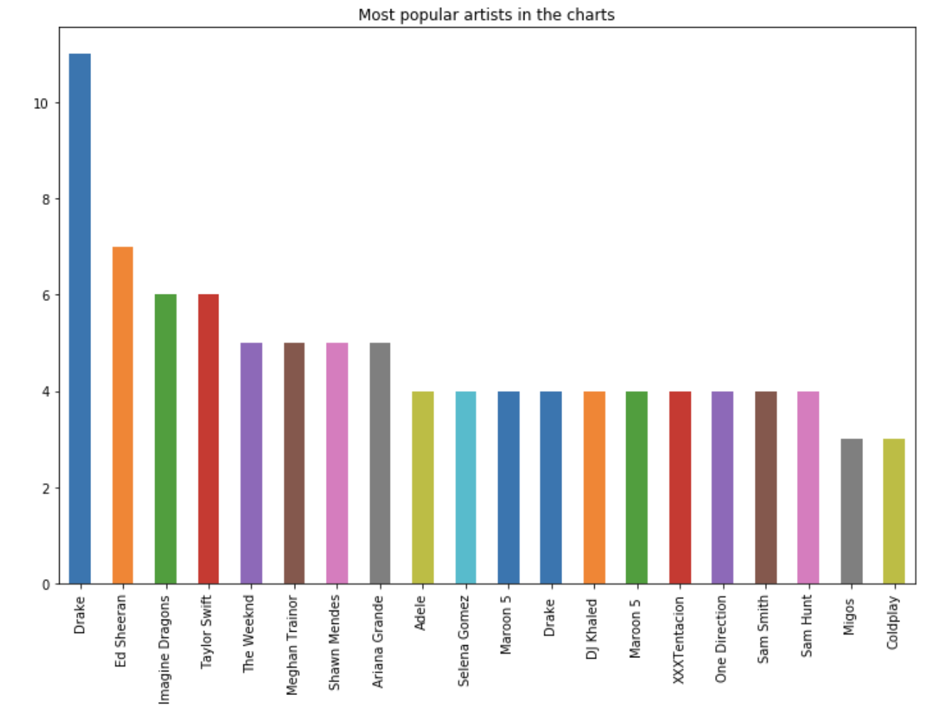
Some artists, like Drake or Ed Sheeran have recorded more hit songs in the time frame considered than any other artist. A song typically has more chances to become a hit if the name of one of those artists is present.

The first model

Now, let’s build a first “benchmark” model that uses the following features :

If there is a featured artist or not
The name of the main artist

This model is a naive benchmark and will rely on a simple decision tree.

from sklearn.model_selection import train_test_split
from sklearn.tree import DecisionTreeClassifier
from sklearn.metrics import f1_score
from sklearn.preprocessing import LabelEncoder

We need to encode the name of the artists into categories to make it understandable for the models we will train :

le = LabelEncoder()
df["Artist_Feat_Num"] = le.fit_transform(df["Artist_Feat"])

Next, we split the X and the y, and create the train and test sets:

X = df[["Artist_Feat_Num", "Featuring"]]
y = df["Hit"]
X_train, X_test, y_train, y_test = train_test_split(X,y, random_state=0) 

We will use a simple decision tree classifier with the default parameters as a benchmark :

dt = DecisionTreeClassifier()
dt.fit(X_train, y_train)
y_pred = dt.predict(X_test)
f1_score(y_pred, y_test)

The resulting F1-score is: 0.066, which is low. The accuracy is close to 86% since our model tends to predict that the song is systematically not a hit. There is room for better data and better models.

Data enrichment through Spotify

Where could we get data from? Well, popular music services like Spotify provide cool APIs that gather a lot of information on artists, albums and tracks. Using external APIs can sometimes be cumbersome. Luckily, there is a great package called Spotipy that does most of the work for us!

Spotipy is available on Github. If you follow the instructions, you will simply have to :

Install the package via PyPI
Create a project from the developer’s console of Spotify
Write down your redirect URI and TokenID
Configure the URI and token in the util file of the package

Let’s move on to the data enrichment. When using Spotipy for the first time, you are required to validate the redirect URI (I have used http://localhost/ ).

import sys
import spotipy
import spotipy.util as util

scope = 'user-library-read'

if len(sys.argv) > 1:
    username = sys.argv[1]
else:
    print("Usage: %s username" % (sys.argv[0],))
sys.exit()

token = util.prompt_for_user_token(username, scope)

It will open an external web page. Simply follow it an copy-paste the URL of the page once logged-in.

Start the Spotipy session :

sp = spotipy.Spotify(auth=token)

sp.trace = True # turn on tracing
sp.trace_out = True # turn on trace out

Spotify’s API has a “search” feature. Type in the name of an artist or a song (or both combined), and it returns a JSON that contains much of the relevant information needed. We will use information from several levels:

The artist: popularity index and the total number of followers. Notice that these values in the API are the values of today, and therefore take into account some information from the future when you compare it to a song published in 2015 for example.
The album: how many songs were there on the album overall, the date of the release, the number of markets it is available in
The song: Spotify has a number of pre-computed features such as speechiness, loudness, danceability and duration.

This will allow us to collect 17 features overall from the Spotify’s API !

def artist_info(lookup) :

    try :
        artist = sp.search(lookup)
        artist_uri = artist['tracks']['items'][0]['album']['artists'][0]['uri']
        track_uri = artist['tracks']['items'][0]['uri']

        available_markets = len(artist['tracks']['items'][0]['available_markets'])
        release_date = artist['tracks']['items'][0]['album']['release_date']

        artist = sp.artist(artist_uri)
        total_followers = artist['followers']['total']
        genres = artist['genres']
        popularity = artist['popularity']

        audio_features = sp.audio_features(track_uri)[0]

        acousticness = audio_features['acousticness']
        danceability = audio_features['danceability']
        duration_ms = audio_features['duration_ms']
        energy = audio_features['energy']
        instrumentalness = audio_features['instrumentalness']
        key = audio_features['key']
        liveness = audio_features['liveness']
        loudness = audio_features['loudness']
        speechiness = audio_features['speechiness']
        tempo = audio_features['tempo']
        time_signature = audio_features['time_signature']
        valence = audio_features['valence']

        return available_markets, release_date, total_followers, genres, popularity, acousticness, danceability, duration_ms, energy, instrumentalness, key, liveness, loudness, speechiness, tempo, time_signature, valence

    except :
        return [None]*17

To enhance our chances to identify the song from the search menu, we will create a feature called “Lookup” that combines the title of the song and the name of the main artist.

df['lookup'] = df['Title'] + " " + df["Artist_Feat"]

Then, apply the function above to create all columns :

df['available_markets'], df['release_date'], df['total_followers'], df['genres'], df['popularity'], df['acousticness'], df['danceability'], df['duration_ms'], df['energy'], df['instrumentalness'], df['key'], df['liveness'], df['loudness'], df['speechiness'], df['tempo'], df['time_signature'], df['valence'] = zip(*df['lookup'].map(artist_info))

The new data frame looks like this :

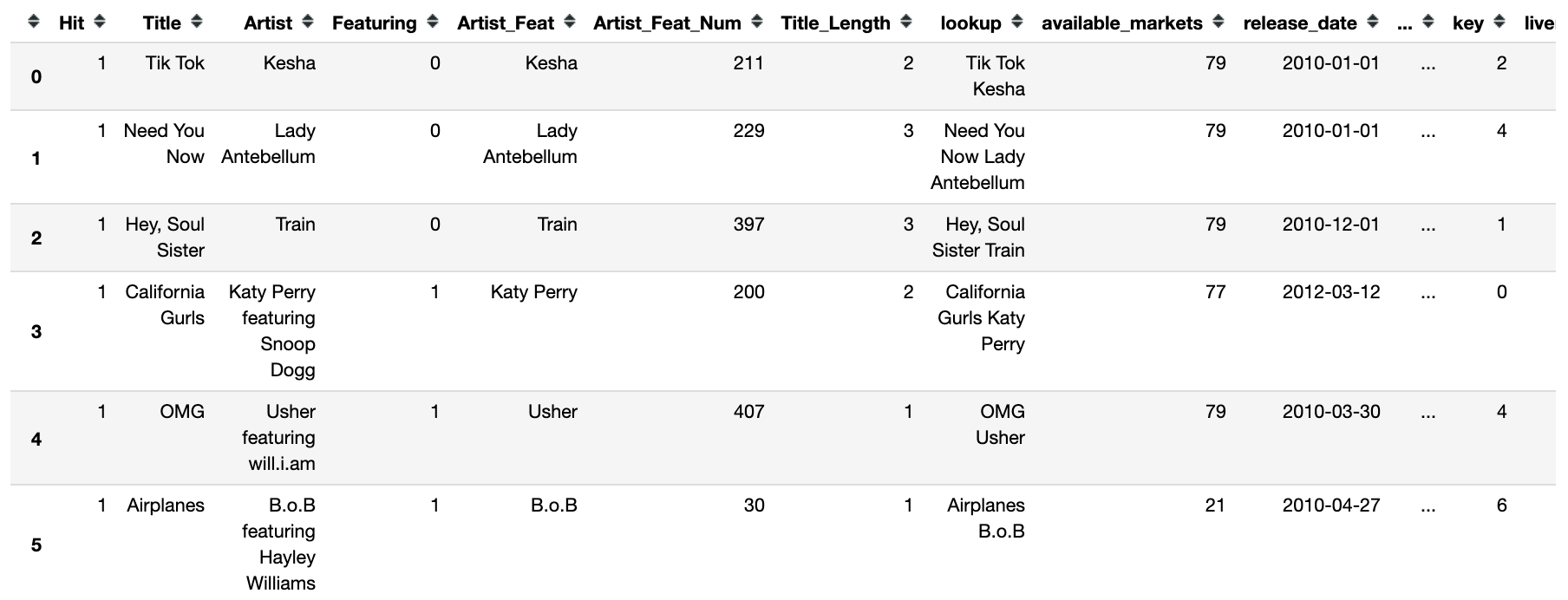
We need to make sure that the API sent back relevant information :

df.shape

(816,25)

df.dropna(how='any').shape

(814,25)

For two of the input songs, we were not able to retrieve the information from the API. We will simply drop those songs :

df = df.dropna()

Not all of the features are exploitable as such. Indeed, the release date is under a date format, which cannot be used as a direct input for a predictive model. We initially specified that we wanted our model not to depend on the year. However, the month of release, the day of the month or even the day of the week might be relevant features.

df['release_date'] = pd.to_datetime(df['release_date'])
df['month_release'] = df['release_date'].apply(lambda x: x.month)
df['day_release'] = df['release_date'].apply(lambda x: x.day)
df['weekday_release'] = df['release_date'].apply(lambda x: x.weekday())

Data Exploration

We now have many features and can proceed to a further data exploration. Let’s start by analyzing the features we just created in relation to the release date:

plt.figure(figsize=(12,8))
plt.hist(df['weekday_release'], bins=14)
plt.title("Weekday release")
plt.show()

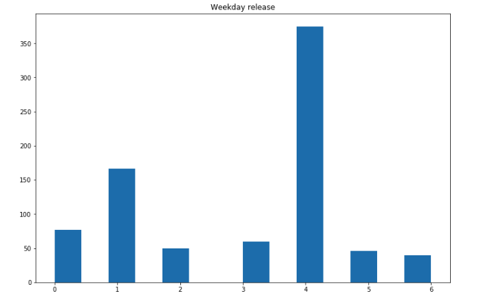
More songs seem to be released on Fridays! That’s an interesting insight.

Regarding the release month :

plt.figure(figsize=(12,8))
plt.hist(df['month_release'], bins=24)
plt.title("Month release")
plt.show()

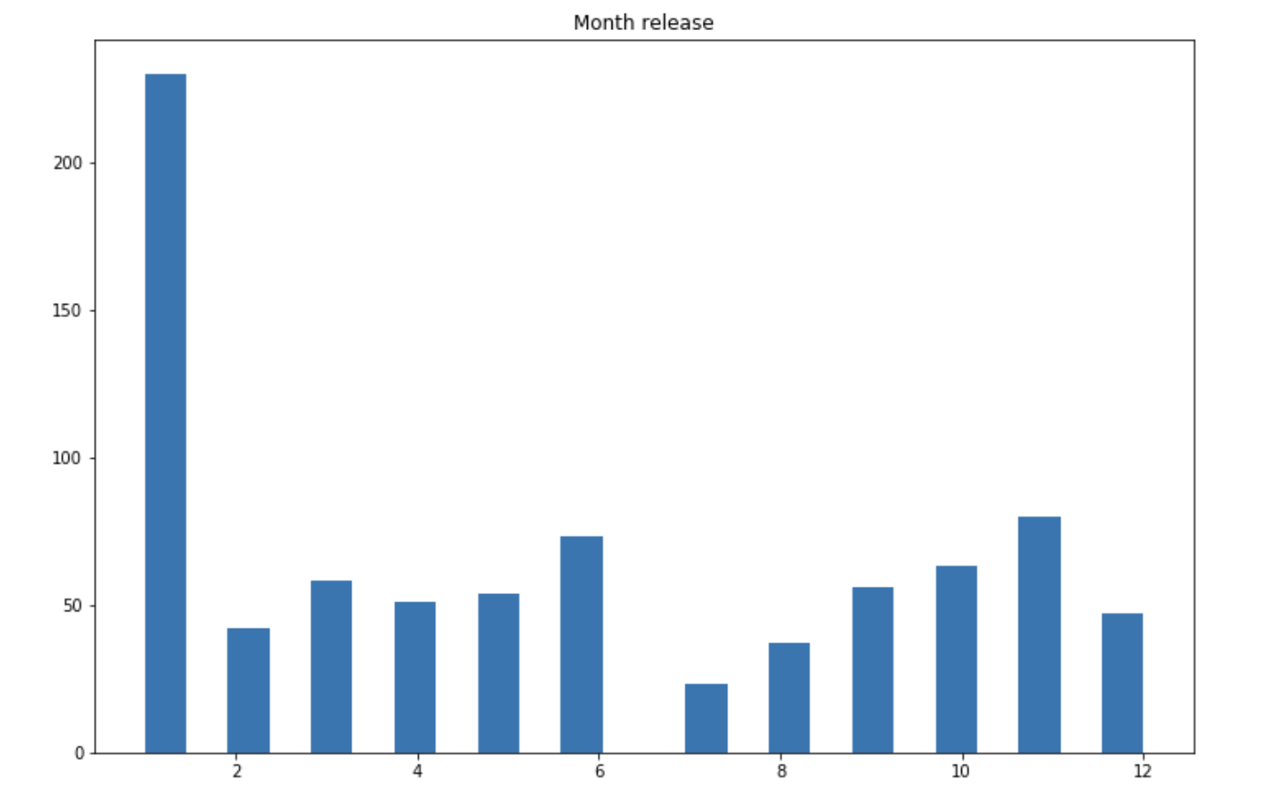
January seems to be a popular choice, although we should probably be careful. Some missing data might be filled by default to January 1st. During the months of July and August, however, there are few songs being released. On the following graph, we see that most songs are available on most markets:

plt.figure(figsize=(12,8))
plt.hist(df['available_markets'], bins=50)
plt.title("Number of markets")
plt.show()

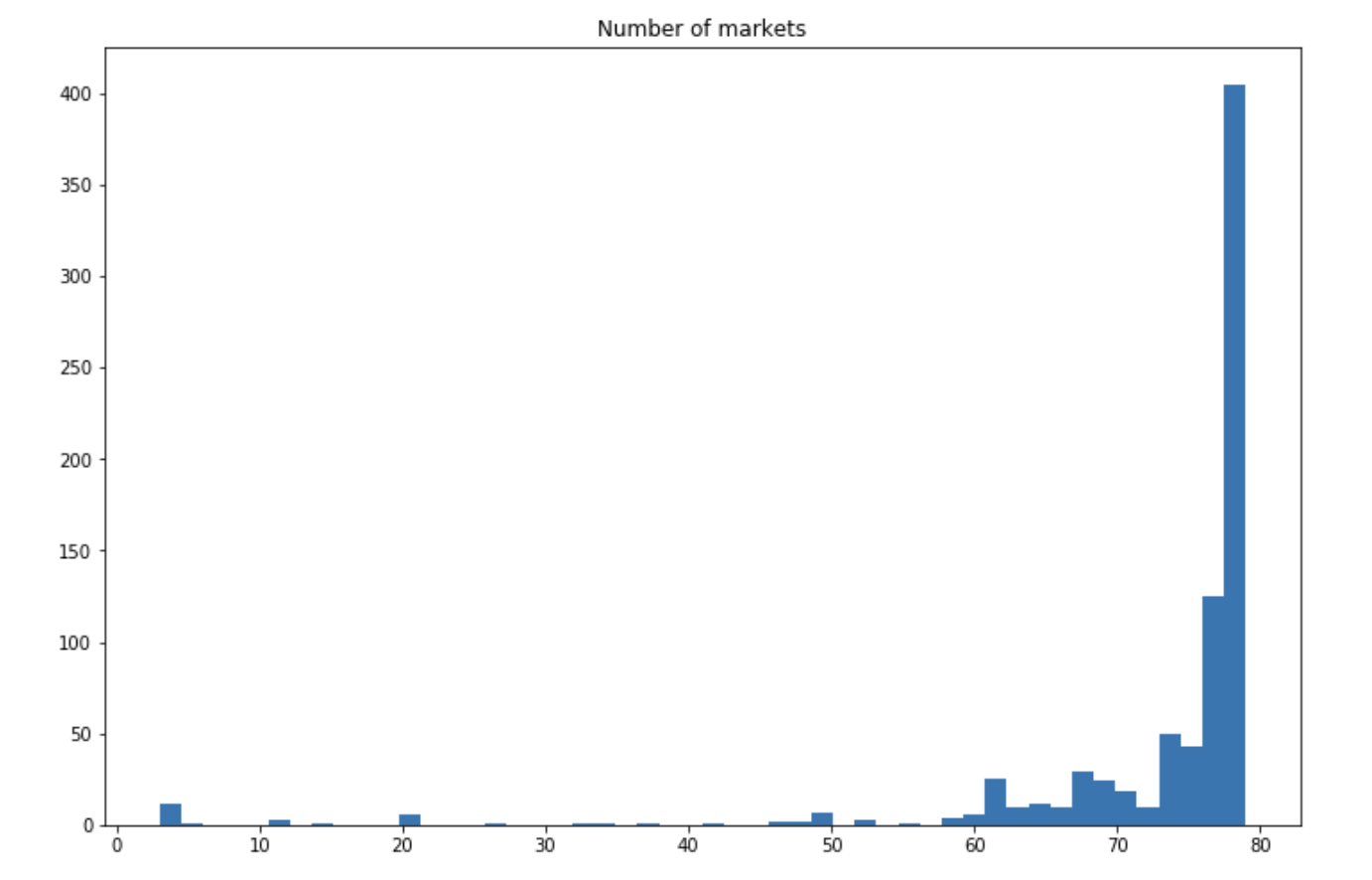
This seems intuitive since a song targeting a large audience has more chances to succeed.

A strong feature will probably be the popularity of the artist :

plt.figure(figsize=(12,8))
plt.hist(df[df['Hit']==1]['popularity'], bins=50, density=True, alpha=0.5, label="Hit")
plt.hist(df[df['Hit']==0]['popularity'], bins=50, density=True, alpha=0.5, label="Not Hit")
plt.title("Artist Popularity")
plt.legend()
plt.show()

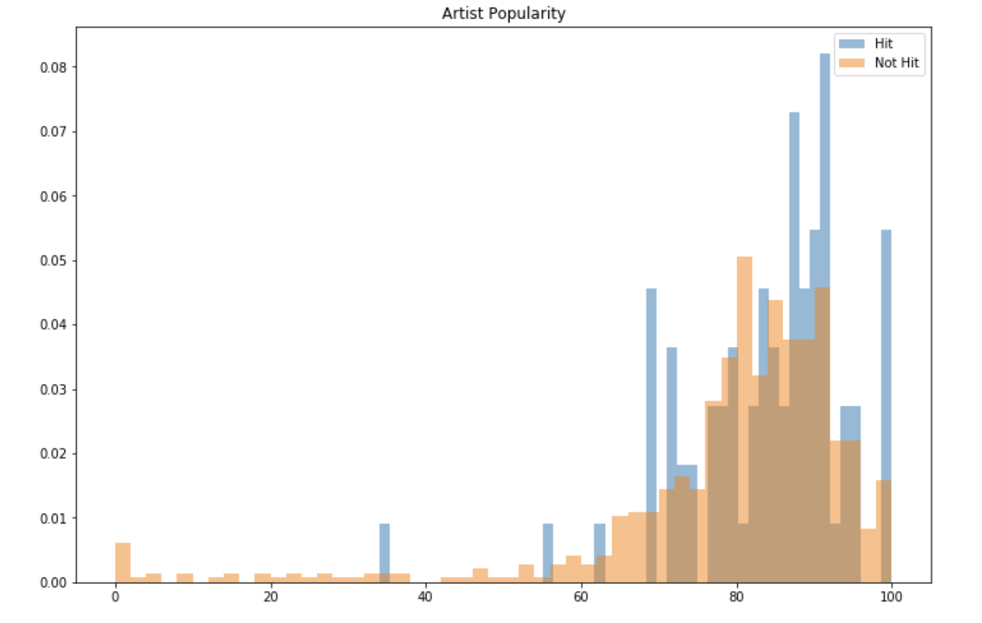
In both cases, the popularity of the artist as defined by Spotify’s API is really high. We however notice that the distribution of the popularity of the artist of hit songs is slightly shifted to the right. On the other hand, several songs that did not become a hit were released by artists with a popularity of less than 70. A really high popularity might be a key feature.

Finally, let’s explore the effect of duration on the hit songs:

plt.figure(figsize=(12,8))
plt.hist(df[df['Hit']==1]['duration_ms'], bins=50, density=True, alpha=0.5, label="Hit")
plt.hist(df[df['Hit']==0]['duration_ms'], bins=50, density=True, alpha=0.5, label="Not Hit")
plt.title("Duration in ms.")
plt.legend()
plt.show()

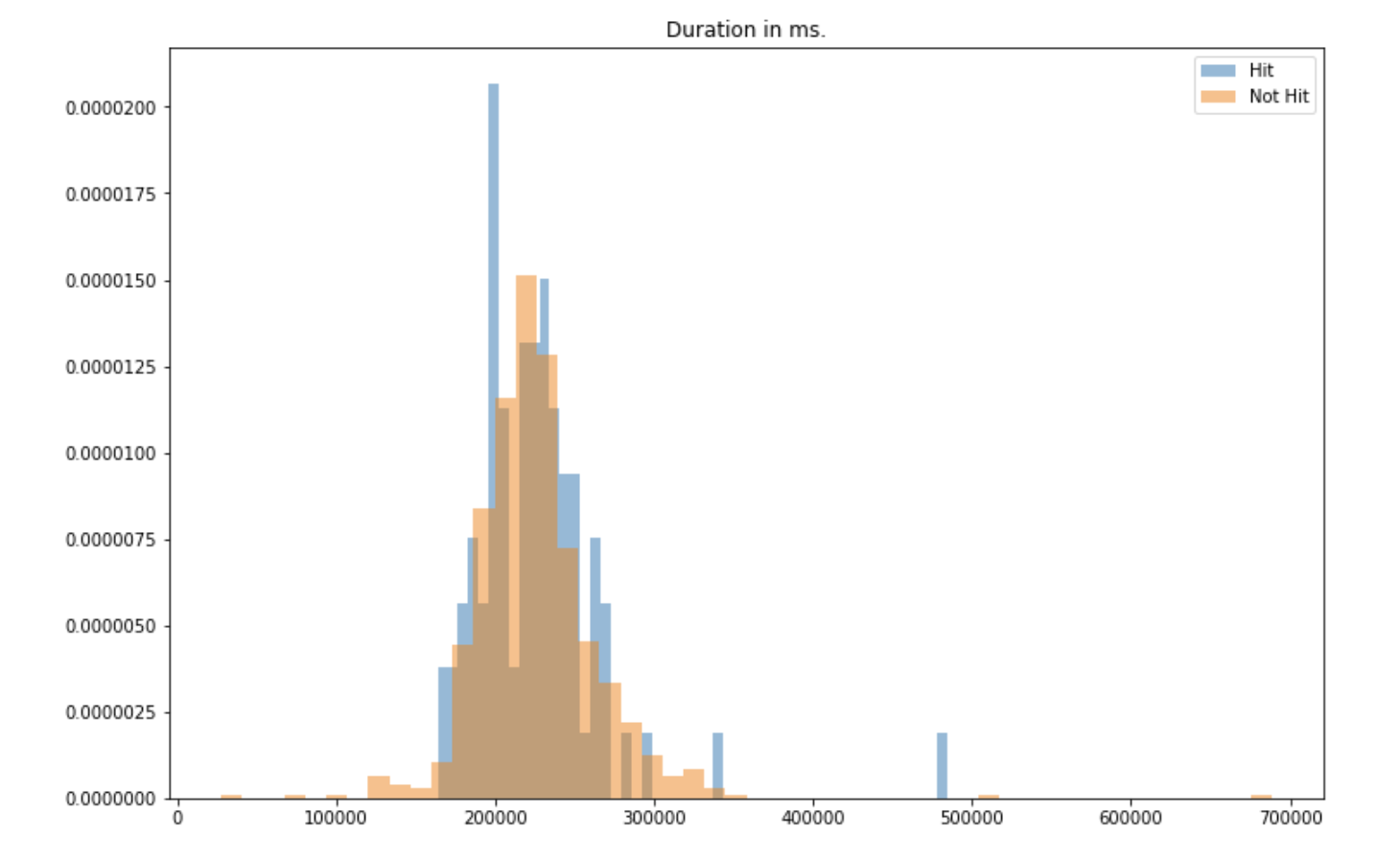
The distribution looks quite similar in both cases. We do not expect the duration of the song to be an important feature.

Same model, better data

We can now build a second classifier. However, we still have quite a limited number of data points and an unbalanced dataset. Can oversampling help?

We will use the Synthetic Minority Over-Sampling Technique (SMOTE). SMOTE is implemented in the package imblearn for Python.

from imblearn.over_sampling import SMOTE

X = df.drop(["Artist_Feat", "Artist", "Artist_Feat_Num", "Title", "Hit", "lookup", "release_date", "genres"], axis=1)
y = df["Hit"]

sm = SMOTE(random_state=42)
X_res, y_res = sm.fit_resample(X, y)
X_train, X_test, y_train, y_test = train_test_split(X_res,y_res, test_size=0.2, random_state=42) 

Let’s apply the same decision tree we used before :

dt = DecisionTreeClassifier(max_depth=100)
dt.fit(X_train, y_train)
y_pred = dt.predict(X_test)
f1_score(y_pred, y_test)

The F1-score reaches 83.4%. Since the data is not unbalanced anymore, we can compute the accuracy:

accuracy_score(y_pred, y_test)

It reaches 84%.

Better model, better data

The decision tree is a good choice for a first model. However, more complex models might improve overall performance. Let’s try this with a Random Forest Classifier :

from sklearn.ensemble import RandomForestClassifier

rf=RandomForestClassifier(n_estimators=100)
rf.fit(X_train, y_train)
y_pred = rf.predict(X_test)

f1_score(y_pred, y_test)

The F1-score reaches 93.3% and the accuracy is 94.5%. Plotting the confusion matrix helps us understand the errors our classifier made :

from sklearn.metrics import confusion_matrix
import seaborn as sns

cm = confusion_matrix(y_test, y_pred)

plt.figure(figsize=(10,8))
sns.heatmap(cm, annot=True)
plt.title("Confusion Matrix")
plt.show()

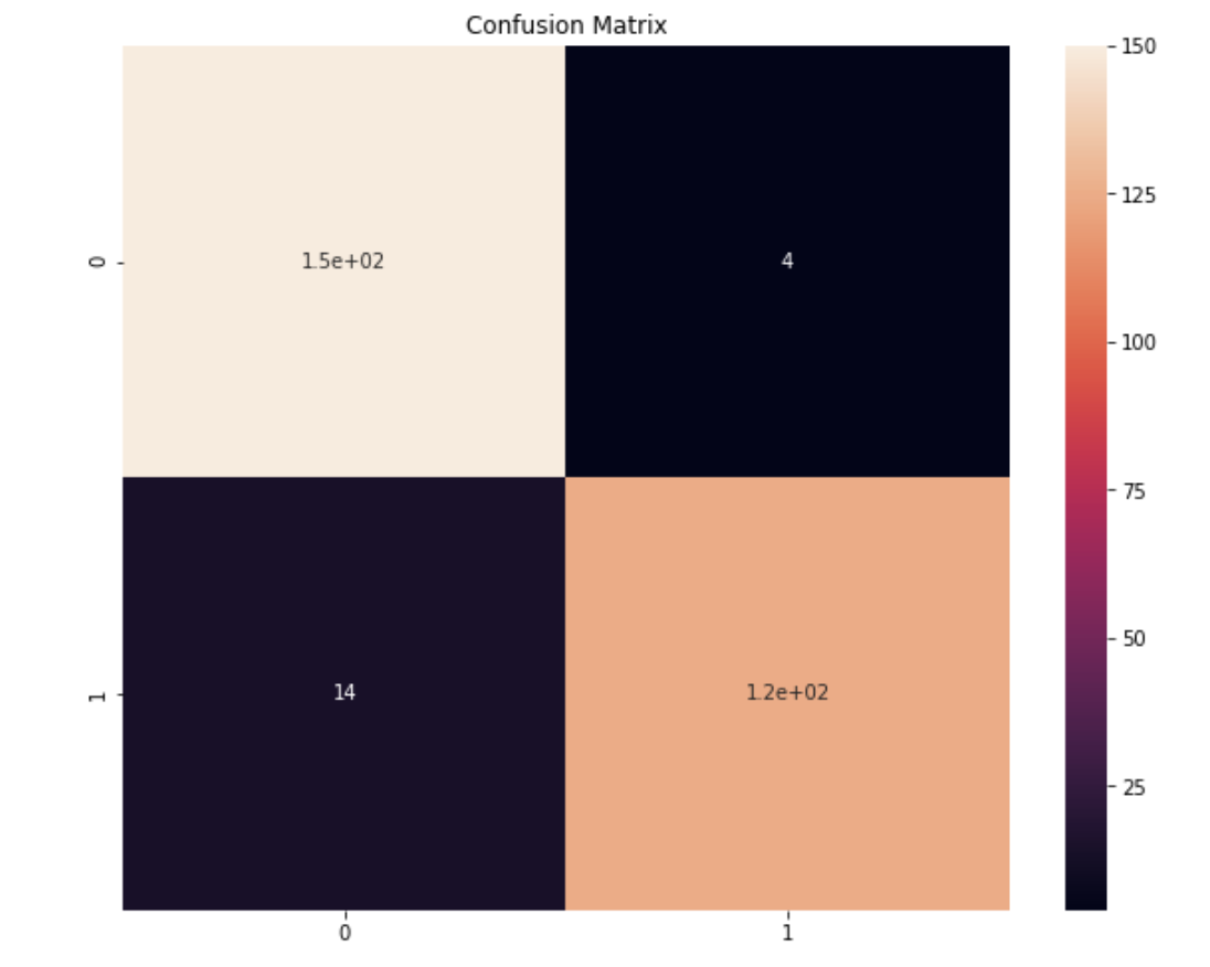
The most common mistake is to have classified a song as a hit whereas it was not (14 cases).

We can now try to understand the output of the classifier by looking at the feature importance :

importances = rf.feature_importances_
indices = np.argsort(importances)

plt.figure(figsize=(12,8))
plt.title('Feature Importances')
plt.barh(range(len(indices)), importances[indices], color='b', align='center')
plt.yticks(range(len(indices)), [X.columns[i] for i in indices])
plt.xlabel('Relative Importance')
plt.show()

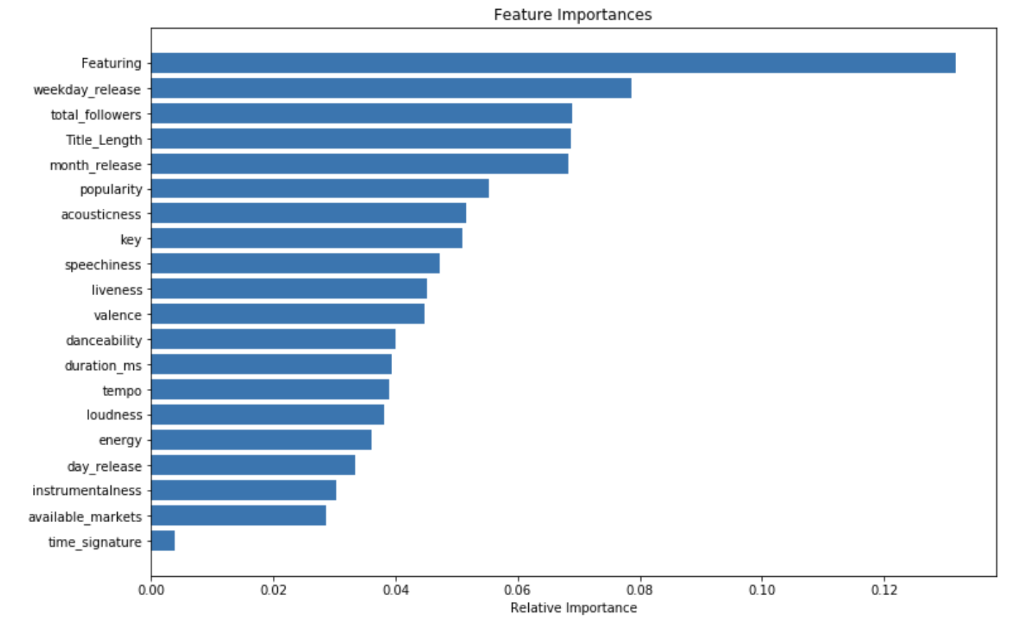
The most important feature is whether there is a featuring artist or not. Then, the most important features are related to the release date, and the popularity of the artist. After that, we find all features related to the song itself.

This analysis highlights something major. Essentially, a song is a hit if it has a good featured artist, is released at the right moment, and the artists who release it are popular. All of this seems logical, but it’s also verified empirically by our model!

Next steps: could we further improve the model by adding the lyrics? We will explore this in the second part of the article.

Predicting the next hit song (Part 1)

Maël Fabien