What is Hyperparameter optimization?

Hyperparameter optimization (HPO) is the process by which we aim to improve the performance of a model by choosing the right set of hyperparameters.

In this article, we will present the main hyperparameter optimization techniques, their implementations in Python, as well as some general guidelines regarding HPO.

In HPO, we generally :

Select a set of hyperparameters to test
Train a model with those hyperparameters on validation data
Evaluate the performance of the model
Move on to the next set of hyperparameters
Keep the hyperparameters which improve the performance the most

There are some major challenges in the field of HPO :

The computation time of a single model with a given set of hyperparameters might be long. Therefore, iterating over many hyperparameter values might be extremely long
The mix of parameters to optimize can be complex, with many parameters, and varying nature (continuous or categorical for example)
There is a risk to overfit on the training set if we aim to ultimately reach the highest performance in the training part
The problem gets even more complex in the field of deep learning

To optimize the hyper-parameters, we tend to use a validation set (if available) to limit the overfitting on the train set.

Let’s illustrate a simple HPO over a simple decision tree. What are the hyperparameters we can impact? You might think of :

criterion
max_depth
min_samples_split
…

How many models should we fit to test all possible combinations of hyperparameters? Well, we can represent the problem graphically :

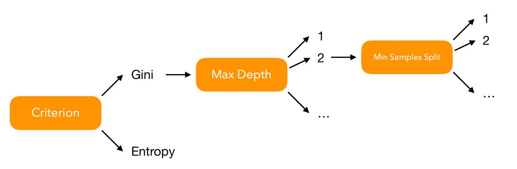
Say that for every hyperparameter \(i\), we have \(V_i\) possible values to test. In that case, over 3 hyperparameters, we face \(V_1 \times V_2 \times V_3\) combinations to test. Over a set of \(P\) hyperparameters, we should test \(\prod_{i=1}^{p} V_i = V_1 \times V_2 \times ... \times V_p\) models.

If we now take into account continuous variables such as a learning rate factor, we rapidly realize that testing all the different hyperparameter combinations is impossible. We need to restrict the space of hyperparameters combinations to look for.

There are two ways to reduce the search space :

Specify a space manually, and explore the space using transparent techniques such as Grid Search or Randomized Search
Use model-based techniques such as Bayesian Hyperparameter Optimization

Grid search and Randomized search are the two most popular methods for hyper-parameter optimization of any model. In both cases, the aim is to test a set of parameters whose range has been specified by the users and observe the outcome in terms of performance of the model. However, the way the parameters are tested is quite different between Grid Search and Randomized Search.

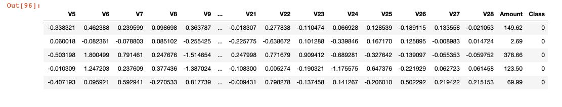
To illustrate the concepts presented below, we will use a Kaggle Credit Card Fraud Detection dataset. The main idea will be to compare the time, the number of combinations tested, the guarantees and the performance of each approach.

The dataset can be found here. It contains transactions made by credit cards in September 2013 by European cardholders. This dataset presents transactions that occurred in two days, where we have 492 frauds out of 284,807 transactions. The dataset is highly unbalanced, the positive class (frauds) account for 0.172% of all transactions.

It contains only numerical input variables which are the result of a PCA transformation. Unfortunately, due to confidentiality issues, the original features are not provided. Features V1, V2, … V28 are the principal components obtained with PCA, the only features which have not been transformed with PCA are ‘Time’ and ‘Amount’. Feature ‘Time’ contains the seconds elapsed between each transaction and the first transaction in the dataset. The feature ‘Amount’ is the transaction Amount, this feature can be used for example-dependant cost-sensitive learning. Feature ‘Class’ is the response variable and it takes value 1 in case of fraud and 0 otherwise.

import pandas as pd
import numpy as np
import matplotlib.pyplot as plt
from sklearn.model_selection import train_test_split

df = pd.read_csv('creditcard.csv')
df.head()

We will use the F1-Score metric, a harmonic mean between the precision and the recall. We will suppose that previous work on the model selection was made on the training set, and conducted to the choice of a Logistic Regression. Therefore, we need to use a validation set to select the right parameters of the logistic regression.

X_train, X_val, y_test, y_val = train_test_split(df.drop(['Class'], axis=1), df['Class'], test_size=0.2)

Grid Search

In grid search, we try every combination of the set of hyperparameters that the user-specified. This means that we will test the following combinations for example :

Criterion	Max Depth	Min Samples Split
Gini	5	2
Gini	5	3
Gini	5	4
Gini	5	5
Gini	10	2
Gini	10	3
Gini	10	4
Gini	10	5
..	..	..
Entropy	50	5

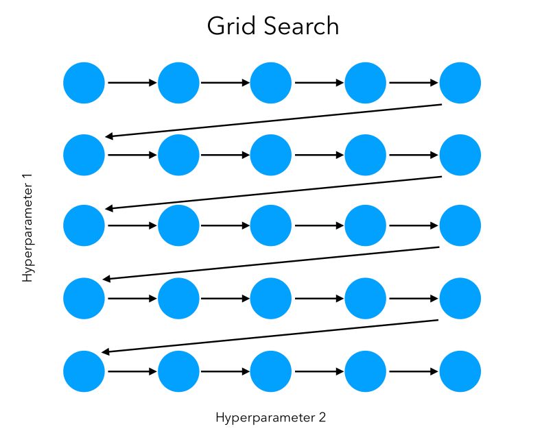
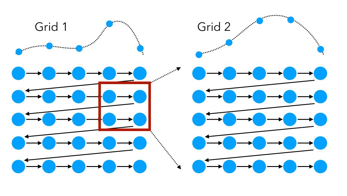
We can visually represent the grid search on 2 features as a sequential way to test, in order, all the combinations:

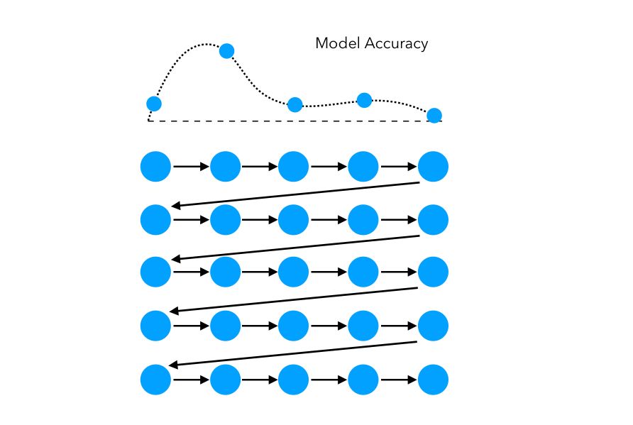
In this simple example, the space explored can be represented as such:

The limitations of grid search are pretty straightforward:

Grid search does not scale well. There is a huge number of combinations we end up testing for just a few parameters. For example, if we have 4 parameters, and we want to test 10 values for each parameter, there are : \(10 \times 10 \times 10 \times 10 = 10'000\) combinations possible.
We have no guarantee to explore the right space.

The user needs a good understanding of the underlying problem to select the right hyperparameters to test. To focus on the right regions of the hyperparameter space, the following technique might be useful:

Start with a first large-scale Grid Search, identify a region of interest in which the models perform well, and start a second Grid Search in this specific region.

This approach can, however, be long to run and should be used if the model you are tuning does not have too many parameters, or if you don’t have too much training data.

Grid search is implemented in scikit-learn under the name of GridSearchCV (for cross-validation):

from sklearn.model_selection import GridSearchCV

param_grid = {
'penalty': ['l1', 'l2'],
'C': [0.8, 1, 1.2], 
'tol': [0.00005, 0.0001, 0.00015, 0.0002], 
'fit_intercept' : [True, False], 
'warm_start' : [True, False]
}

lr = LogisticRegression()
grid_search = GridSearchCV(lr, param_grid, cv=5, scoring='f1_macro', return_train_score=True)
grid_search.fit(X_val, y_val)

After approximately 4 minutes, the best model appears to be the following:

estimator=LogisticRegression(C=1.0, class_weight=None, dual=False, fit_intercept=True,
intercept_scaling=1, max_iter=100, multi_class='warn',
n_jobs=None, penalty='l2', random_state=None, solver='warn',
tol=0.0001, verbose=0, warm_start=False)

To access the results and the details of the GridSearch Cross-Validation, simply use:

grid_search.cv_results_ 

This gives access to the fitting time, the prediction time, the training score, the test score… The average F1-Score on the test set of the Cross Validations can be computed by taking the mean of the test scores array:

np.mean(grid_search.cv_results_['mean_test_score'])

We achieve an average F1-Score of approximately 0.837 in 4 minutes and 17 seconds.

Randomized Search

The randomized search follows the same goal. However, we won’t test sequentially all the combinations. Instead, we try random combinations among the range of values specified for the hyper-parameters. We initially specify the number of random configurations we want to test in the parameter space.

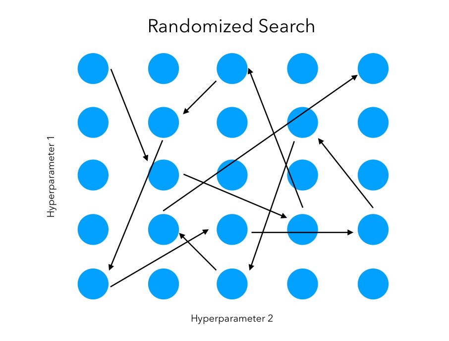
The main advantage is that we can try a broader range of values or hyperparameters within the same computation time as grid search, or test the same ones in much less time. We are however not guaranteed to identify the best combination since not all combinations will be tested.

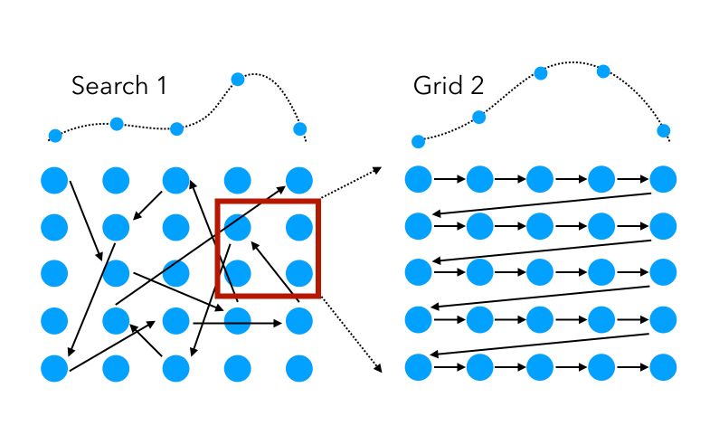
To get back to our previous example in which we used 2 successive hyperparameter techniques in a row, randomized Search can also be used as the first layer, to either speed up the process on the same set of hyperparameters, or explore a broader range of feature values.

Mathematically, for a given number of iterations (function evaluations), say \(N\) in total, on a set of \(V\) hyperparameters :

A grid search will explore \(N^{\frac{1}{V}}\) values for each hyperparameter
Whereas a randomized search will explore \(N\) different values for each hyperparameter

The implementation in Scikit-learn is also straight forward :

from sklearn.model_selection import RandomizedSearchCV

param_grid = {
'penalty': ['l1', 'l2'],
'C': [0.8, 1, 1.2], 
'tol': [0.00005, 0.0001, 0.00015, 0.0002], 
'fit_intercept' : [True, False], 
'warm_start' : [True, False]
}

lr = LogisticRegression()
rnd_search = RandomizedSearchCV(lr, param_grid, n_iter = 20, cv=5, scoring='f1_macro', return_train_score=True)
rnd_search.fit(X_val, y_val)

The optimal model identified is exactly the same:

estimator=LogisticRegression(C=1.0, class_weight=None, dual=False, fit_intercept=True,
intercept_scaling=1, max_iter=100, multi_class='warn',
n_jobs=None, penalty='l2', random_state=None, solver='warn',
tol=0.0001, verbose=0, warm_start=False)

The average F1-Score is quite similar, although there is a slight difference due to the Cross Validation split. We managed to successfully explore the combination of parameters in less than 53 seconds. In this example, the randomized search was successful, but it’s not always the case.

There is a tradeoff to make between the guarantee to identify the best combination of parameters and the computation time. As mentioned, a simple trick could be to start with a randomized search to reduce the parameters space and then launch a grid search to select the optimal features within this space.

The main limit of Grid Search or Randomized Search is that the point we just explored does not influence which point to evaluate next since these two approaches do not depend on an underlying model. To overcome this limitation, we will introduce Bayesian Hyperparameter Optimization

Bayesian Hyperparameter Optimization

Bayesian Hyperparameter Optimization is a model-based hyperparameter optimization, in the sense that we aim to build a distribution of the loss function in terms of the value of each parameter. What are the main advantages and limitations of model-based techniques? How can we implement it in Python?

Recall that in an optimization problem regarding a model’s hyperparameters, the aim is to identify :

\[x^* = argmin_x f(x)\]

where \(f\) is an expensive function.

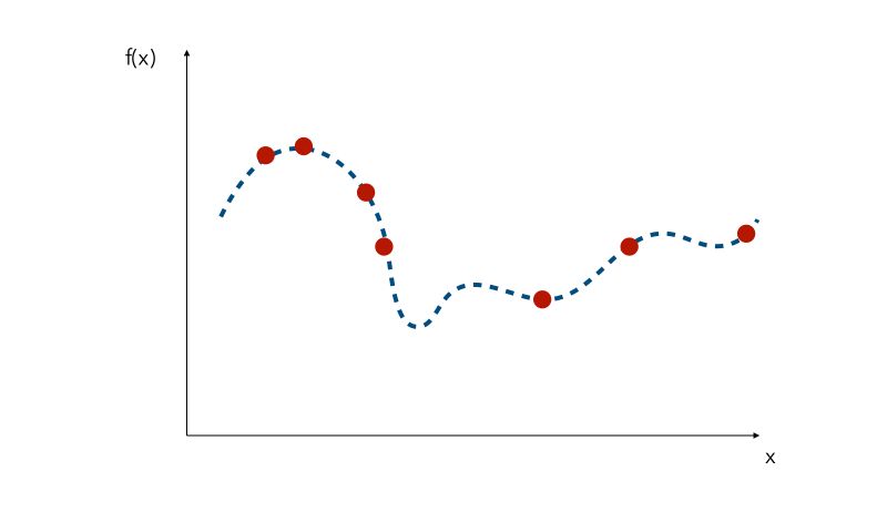
Depending on the form or the dimension of the initial problem, it might be really expensive to find the optimal value of \(x\). Hyperparameter gradients might also not be available. Suppose that we know all the parameters distribution. We can represent for every hyperparameter, a distribution of the loss according to its value.

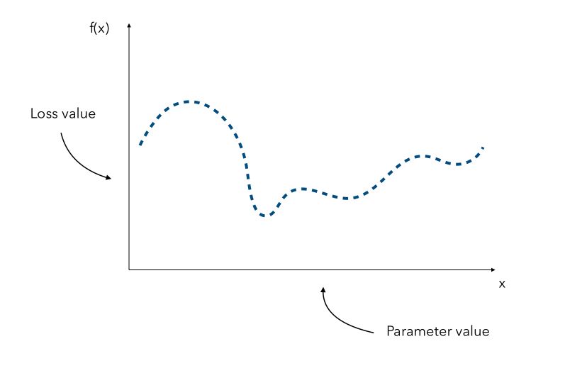
Since the curve is not known, a naive approach would be the pick a few values of x and try to observe the corresponding values f(x). We would then pick the value of x that gave the smallest value.

This is where Grid Search and Randomized search lie, and all other similar methods are called Sequential model-based optimization (SMBO).

Probabilistic Regression Models

We try to approximate the underlying function using only the samples we have. This can essentially be done in 2 steps :

identify a probabilistic surrogate model, i.e. a model that describes the distribution the loss in terms of the underlying hyperparameter value
define an acquisition function which tells us which point to explore next

Surrogate models

Although Random Forest and Tree Parzen Estimators (TPE) are quite popular choices, we will focus on Gaussian Processes (GP) for surrogate models.

We suppose that the function \(f\), which represents the distribution of a loss in terms of the value of a hyperparameter, has a mean \(\mu\) and a covariance \(K\), and is a realization of a Gaussian Process. The Gaussian Process is a tool used to infer the value of a function. Predictions follow a normal distribution. Therefore :

\[p(y \mid x, D) = N(y \mid \hat{\mu}, {\hat{\sigma}}^2)\]

We use that set of predictions and pick new points where we should evaluate next. We can plot a Gaussian Process between 4 samples this way :

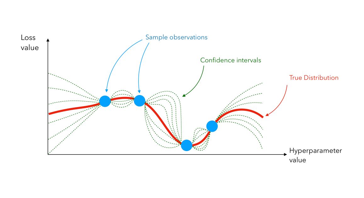
Even though the true distribution is unknown (the red line), we can infer its value using Gaussian Process (confidence interval lines in green).

Once we identify a new point using the acquisition function, we add it to the samples and re-build the Gaussian Process with that new information… We keep doing this until we reach the maximal number of iterations or the limit time for example. This is an iterative process.

Acquisition function

How do we know which point we should evaluate next? There are two guidelines :

Pick points that yield, on the approximated curve, a low value.
Pick points in areas we have less explored.

There is an exploration/exploitation trade-off to make. This tradeoff is taken into account in an acquisition function.

The acquisition function is defined as :

\[A(x) = \sigma(x) ( \gamma(x) \Phi( \gamma(x)) + N (\gamma(x)))\]

where :

\[\gamma(x) = \frac { f(x^c) - \mu(x)} {\sigma(x)}\]
\(f(x^c)\) the current guessed arg min, \(\mu(x)\) the guessed value of the function at x, and \(\sigma(x)\) the standard deviation of output at x.
\(\Phi(x)\) and \(N(x)\) are the CDF and the PDF of a standard normal

This acquisition function is the most common and is called the expected improvement. We then compute the acquisition score of each point, pick the point that has the highest activation, and evaluate \(f(x)\) at that point, and so on…

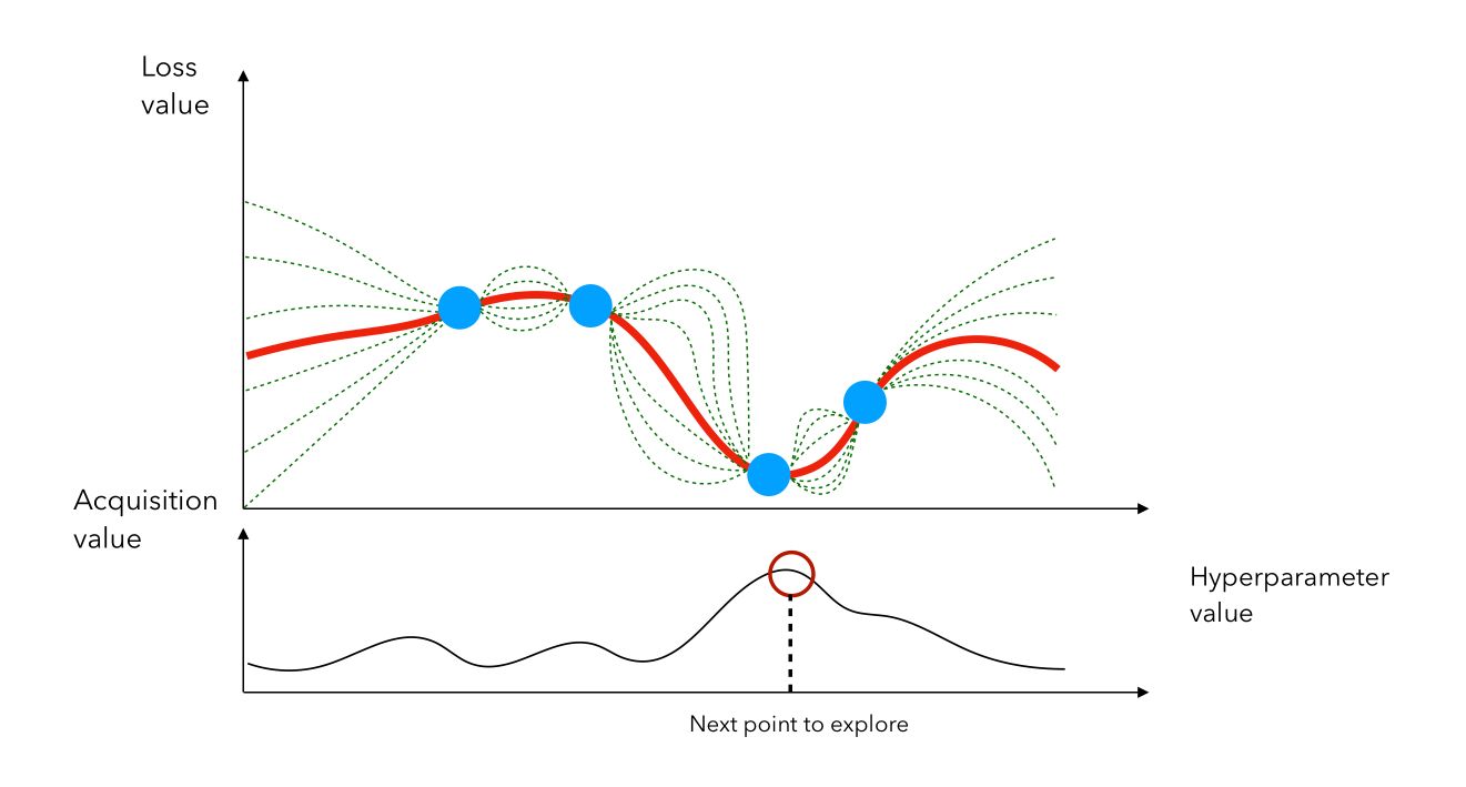
In this example, we would stay in the region in which we identified a previous point that gave a small loss. We can also see the loss minimization problem as a maximization problem on the chosen metric.

The gaussian hyperparameter optimization process can be illustrated in the following way :

This is the essence of bayesian hyperparameter optimization!

Advantages and limits of Bayesian Hyperparameter Optimization

Bayesian optimization techniques can be effective in practice even if the underlying function \(f\) being optimized is stochastic, non-convex, or even non-continuous.

Bayesian optimization is effective, but it will not solve all our tuning problems. As the search progresses, the algorithm switches from exploration — trying new hyperparameter values — to exploitation — using hyperparameter values that resulted in the lowest objective function loss.

If the algorithm finds a local minimum of the objective function, it might concentrate on hyperparameter values around the local minimum rather than trying different values located far away in the domain space. Random search does not suffer from this issue because it does not concentrate on any values!

Implementation in Python

Several libraries implement Gaussian Hyperparameter Optimization and rely on different theoretical aspects of this HPO method.

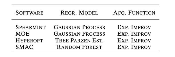
We will be using HyperOpt in this example since it’s one of the most famous HPO libraries in Python, that can also be used for Deep Learning.

HyperOpt

Import the HyperOpt packages and functions :

from hyperopt import tpe
from hyperopt import STATUS_OK
from hyperopt import Trials
from hyperopt import hp
from hyperopt import fmin

In this example, we will try to optimize the Logistic Regression. Define the maximum number of evaluations and the maximum number of folds :

N_FOLDS = 10
MAX_EVALS = 50

We start by defining an objective function, i.e the function to minimize. Here, we want to maximize the cross-validation F1 Score, and therefore minimize 1 - CV(F1-Score) :

def objective(params, n_folds = N_FOLDS):
"""Objective function for Logistic Regression Hyperparameter Tuning"""

# Perform n_fold cross validation with hyperparameters
clf = LogisticRegression(**params,random_state=0,verbose =0)
scores = cross_val_score(clf, X_val, y_val, cv=5, scoring='f1_macro')

# Extract the best score
best_score = max(scores)

# Loss must be minimized
loss = 1 - best_score

# Return all relevant information
return {'loss': loss, 'params': params, 'status': STATUS_OK}

Then, we define the space, i.e the range of all parameters we want to tune :

space = {
'warm_start' : hp.choice('warm_start', [True, False]),
'fit_intercept' : hp.choice('fit_intercept', [True, False]),
'tol' : hp.uniform('tol', 0.00001, 0.0001),
'C' : hp.uniform('C', 0.05, 3),
'solver' : hp.choice('solver', ['newton-cg', 'lbfgs', 'liblinear', 'sag', 'saga']),
}

Notice that we won’t be able to compute the number of combinations tested here since we use uniform distributions for continuous variables such as C and the tolerance tol. We will limit the number of trials to 50 instead, as defined by MAX_EVALS. We are now ready to run the optimization :

tpe_algorithm = tpe.suggest
bayes_trials = Trials()
best = fmin(fn = objective, space = space, algo = tpe.suggest, max_evals = MAX_EVALS, trials = bayes_trials)

You’ll see the progress similarly:

90%|█████████ | 45/50 [05:09<00:31, 6.21s/it, best loss: 0.06831375590721178]

The variable best contains the model with the best parameters.

{'C': 1.602432793095192,
'fit_intercept': 0,
'solver': 1,
'tol': 9.914353259315055e-05,
'warm_start': 1}

The best solution identified is now different since we explored continuous distributions for several parameters.

Conclusion

The following table summarizes the performance of the different approaches:

Method	Time	Combinations tested	CV F1-Score
Grid Search	4m 17s	96	0.837307
Randomized Search	53s	20	0.843494
Bayesian Optimization	5m58s	50	0,931686

We notice that the bayesian optimization outperforms the two other approaches, and can be longer eventually. We tested more combinations of the grid search, but identifying optimal parameters as precise as the ones in bayesian optimization would have required a lot more of combinations for the grid search and the randomized search.

The randomized search achieved results similar to grid search, in less than 25% of the computation time. The identification of the optimal set of hyperparameters is however not guaranteed. It is possible to specify a broader set of parameters to test in grid search and randomized search using np.arange function, but the underlying distribution remains discrete.

In conclusion, using the Bayesian approach seems to be a good choice, since it can learn complex relations and interactions between the hyperparameters. There is however a risk that such an approach focuses only on local minima, and controlling this with a randomize search at first might be a good idea.

Sources :

A Guide to Hyperparameter Optimization (HPO)

Maël Fabien