Who’s the painter ?

In this article, we will be using data from the Web Gallery of Art, a virtual museum and searchable database of European fine arts from the \(3^{rd}\) to \(19^{th}\) centuries. The gallery can be accessed here.

We will create an algorithm to predict the name of the painter based on an intial set of features of the painting, and then gradually including more and more, thus improving the feature engineering, and including pictures.

Through this article, we will illustrate:

• The importance of good feature engineering;
• The importance of data enrichment; and
• The impact this can have on accuracy

Ready ? Let’s get started !

The data

To download the data, you can either :

• click on this link to download the XLS file directly
• go to Database tab in the website, and click on the last link : You can download the catalogue for studying or searching off-line. Select the Excel format of 5.2 Mb.

Start off by importing several packages to be used later:

### Manipulating and plotting data ###
import pandas as pd
import numpy as np
import matplotlib.pyplot as plt
import matplotlib.image as mpimg
import seaborn as sns

### Process text ###
from nltk.corpus import stopwords
from nltk.tokenize import word_tokenize
import spacy
from sklearn.decomposition import PCA
from sklearn.preprocessing import MinMaxScaler
import re
nlp = spacy.load('en_core_web_md')

### Process images ###
import glob
import cv2
import matplotlib.image as mpimg
import urllib.request
from sklearn.preprocessing import StandardScaler

### Modeling libraries performance ###
from sklearn import preprocessing
from sklearn.metrics import accuracy_score
from sklearn.metrics import confusion_matrix
from sklearn.model_selection import cross_val_predict
from sklearn.model_selection import cross_val_score
from sklearn.ensemble import RandomForestClassifier

import warnings
warnings.filterwarnings("ignore")

The architecture of our folders should be the following:

- Notebook.ipynb
- images
- catalog.xlsx

Images is an empty folder to be used later.

Import the file catalog.xlsx :

catalog = pd.read_excel('catalog.xlsx', header=0)
catalog.head()

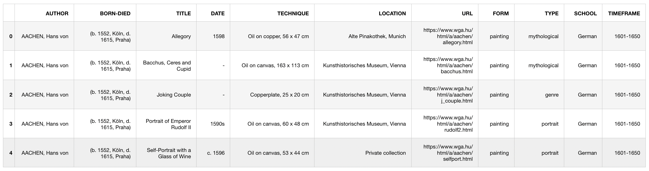
We directly notice that we need to process the data, to make it exploitable. The available columns are :

• The author, which we will try to predict
• The date of birth and death of the author. We will drop this column since it is directly linked to the author
• The title of the painting
• The date of the painting, if available
• The technique used (Oil on copper, oil on canvas, wood, etc) as well as the size of the painting
• The current location of the painting
• The URL of the image on the website
• The form (painting, ceramics, sculpture, etc). We will only focus on paintings in our case.
• The type of painting (mythological, genre, portrait, landscape, etc.)
• The school, i.e. the dominant painting style
• The timeframe in which experts estimate that the painting was painted

Feature engineering

Since the dataset itself is not made for running a ML algorithm, but meant to be a simple catalog, we need some processing.

Date

By exploring the data, we notice missing values for the date. When the date is approximative, it is denoted by :

• 1590s
• or c.1590

Moreover, the missing values are denoted by a hyphen. For all these reasons, using a regex to extract the date seems to be appropriate.

def date_extract(date) :
    try :
        return re.findall('\d+', date)[0]
    except :
        return None

catalog['DATE'] = catalog['DATE'].astype(str)
catalog['DATE'] = catalog['DATE'].apply(lambda x : date_extract(x))

The time frame is redundant if the date is known. Including both variables would imply adding multi-colinearity in the data.

catalog = catalog.drop(['TIMEFRAME'], axis=1)

Technique

The “Technique” is an interesting feature. It is a string that takes the following form:

Oil on copper, 56 x 47 cm

We can extract several elements from this feature:

• The type of painting (oil on copper)
• The height
• The width

We will only focus on paintings, and drop observations that are sculplures or architecture for example.

catalog = catalog[catalog['FORM'] == 'painting']

We can apply several functions to extract the width and height:

def height_extract(tech) :
    try :
        return re.findall('\d+', tech.split(" x ")[0])[0]
    except :
        return None

def width_extract(tech) :
    try :
        return re.findall('\d+', tech.split(" x ")[1])[0]
    except :
        return None
        
catalog['HEIGHT'] = catalog['TECHNIQUE'].apply(lambda x : height_extract(x))
catalog['WIDTH'] = catalog['TECHNIQUE'].apply(lambda x : width_extract(x))

Width and height

In some cases, the “Technique” feature does not contain the width nor the height. We might want to fill the missing values. It’s not a good idea to fill it with 0’s. To minimize the error, we’ll set the missing values to the average of each feature.

catalog['HEIGHT'] = catalog['HEIGHT'].fillna(0).astype(int)
catalog['WIDTH'] = catalog['WIDTH'].fillna(0).astype(int)

mean_height = sum(catalog[catalog['HEIGHT']>0]['HEIGHT'])/len(catalog[catalog['HEIGHT']>0]['HEIGHT'])
mean_width = sum(catalog[catalog['WIDTH']>0]['WIDTH'])/len(catalog[catalog['WIDTH']>0]['WIDTH'])

def treat_height(height) :
    if height == 0 :
        return mean_height
    else : 
        return height

def treat_width(width) :
    if width == 0 :
        return mean_width
    else : 
        return width

catalog['HEIGHT'] = catalog['HEIGHT'].apply(lambda x : treat_height(x))
catalog['WIDTH'] = catalog['WIDTH'].apply(lambda x : treat_width(x))

Missing values and useless columns

As stated above, we won’t exploit the birth nor death of the author, since it’s an information that depends on the author.

catalog = catalog.drop(['BORN-DIED'], axis=1)

At this point we can confidently drop any row that has missing values since the processing is almost over.

catalog = catalog.dropna()

There are many authors in the database (> 3500). To check this, simply run a values count on the author’s feature.

catalog['AUTHOR'].value_counts()

We will need a good number of training samples for each label for the algorithm to be applied. For this reason, all authors with less than 200 observations should be dropped. This is a major limitation in our simple model, but will give a better class balance later on.

counts = catalog['AUTHOR'].value_counts()
catalog = catalog[catalog['AUTHOR'].isin(counts.index[counts > 200])]
catalog['AUTHOR'].value_counts()

GIOTTO di Bondone                 564
GOGH, Vincent van                 332
REMBRANDT Harmenszoon van Rijn    315
RUBENS, Peter Paul                303
RAFFAELLO Sanzio                  289
TINTORETTO                        287
MICHELANGELO Buonarroti           278
CRANACH, Lucas the Elder          275
TIZIANO Vecellio                  269
VERONESE, Paolo                   266
TIEPOLO, Giovanni Battista        249
GRECO, El                         245
ANGELICO, Fra                     242
UNKNOWN MASTER, Italian           236
MEMLING, Hans                     209
BRUEGEL, Pieter the Elder         205

A first model

The aim of this exercise is to illustrate the need for a good feature engineering and additional data. We won’t spend too much time on the optimization of the model itself and we will use a random forest classifier. A label encoding needs to be applied to transform the labels into numeric values that can be understood by our model.

The accuracy of a model will be evaluated by the average of the cross validation with 5 folds.

df = catalog.copy()
df = df.drop(['TITLE', 'LOCATION', 'TECHNIQUE', 'URL'], axis=1)

le = preprocessing.LabelEncoder()

df['AUTHOR'] = le.fit_transform(df['AUTHOR'])
df['FORM'] = le.fit_transform(df['FORM'])
df['TYPE'] = le.fit_transform(df['TYPE'])
df['SCHOOL'] = le.fit_transform(df['SCHOOL'])

rf = RandomForestClassifier(n_estimators=500)
y = df['AUTHOR']
X = df.drop(['AUTHOR'], axis=1)

cv = cross_val_score(rf, X, y, cv=5)
print(cv)  
print(np.mean(cv))

[0.79623477 0.81818182 0.86399108 0.87150838 0.70594837]
0.8111728850092941

The mean accuracy during our cross validation reaches 81.1% with our simple random forest model. We can also look at the confusion matrix.

y_pred = cross_val_predict(rf, X, y, cv=5)
conf_mat = confusion_matrix(y, y_pred)

plt.figure(figsize=(12,8))
sns.heatmap(conf_mat)
plt.title("Confusion Matrix")
plt.show()

It’s easy to understand that mistakes are made more frequently with latest authors, given that we have fewer observations for these.

More feature engineering

Technique

Alright, we are now ready to move on and add other variables by improving the feature engineering. Looking at the “Technique” feature, you will notice that we have not used the “type of painting” variable yet. Indeed, only the width and height have been extracted from this field.

The technique is systematically specified before the first comma. We will split the string on the first comma, if there is one, and then select the first word (oil, tempera, wood…).

def process_tech(tech) :
    tech = tech.split(" ")[0]
    try : 
        return tech.split(",")[0]
    except :
        return tech

catalog['TECHNIQUE'] = catalog['TECHNIQUE'].apply(lambda x: process_tech(x))

Location

So far we have not exploited the location field either. The location describes where the painting is being kept. We only extract the name of the city from this field as extracting the name of the museum would lead to an overfitting. The collections of each museum are limited, and we only have at this point around 4’500 training samples.

def process_loc(loc) :
    return loc.split(",")[-1]
    
catalog['LOCATION'] = catalog['LOCATION'].apply(lambda x: process_loc(x))

Second model

After adding these two variables, we can test again the outcome on a cross validation.

df = catalog.copy()
df = df.drop(['TITLE', 'URL'], axis=1)

le = preprocessing.LabelEncoder()

df['AUTHOR'] = le.fit_transform(df['AUTHOR'])
df['TECHNIQUE'] = le.fit_transform(df['TECHNIQUE'])
df['FORM'] = le.fit_transform(df['FORM'])
df['TYPE'] = le.fit_transform(df['TYPE'])
df['SCHOOL'] = le.fit_transform(df['SCHOOL'])
df['LOCATION'] = le.fit_transform(df['LOCATION'])
df['TECH'] = le.fit_transform(df['TECH'])

y = df['AUTHOR']
X = df.drop(['AUTHOR'], axis=1)

Then, run the cross validation :

cv = cross_val_score(rf, X, y, cv=5)
print(cv)  
print(np.mean(cv))

[0.83277962 0.83037694 0.88963211 0.88938547 0.7620651 ]
0.8408478481785021

And print the confusion matrix :

y_pred = cross_val_predict(rf, X, y, cv=5)
conf_mat = confusion_matrix(y, y_pred)

plt.figure(figsize=(12,8))
sns.heatmap(conf_mat)
plt.title("Confusion Matrix")
plt.show()

We have gained a significant accuracy by improving the feature engineering !

Process the title

Can the processing of the title bring additional accuracy ? It might be interesting to :

• Embed the title using a pre-trained model
• Reduce the dimension of the embedding using a Principal Component Analysis (PCA)
• Use the new dimensions as new features to predict the name of the painter

To start, download pre-trained models from Spacy from your terminal :

python -m spacy download en_core_web_md

We will be using a pre-trained Word2Vec model and begin by defining the embedding function:

def embed_txt(titles) :
    list_mean = []

    # For each title
    for title in titles :
    
        # Tokenize the title
        tokens = word_tokenize(title)
        all_embedding = []
        arr = np.empty((300,))

        # Compute the embedding of each word
        for token in tokens :
            arr = np.append(arr, np.array(nlp(token).vector), axis=0)     
        
        # Compute the average embedding of the title
        arr = arr.reshape(300, -1)
        arr = np.nan_to_num(arr)
        mean = np.mean(arr, axis = 1)
        list_mean.append(mean)

    return list_mean

We then apply our function to the list of titles :

embedding = np.array(embed_txt(list(catalog['TITLE'])))

We will now reduce the dimension (300 currently) of the embedding to use it as features in our prediction. The Principal Component Analysis (PCA) is sensitive to scaling, and requires a scaling of the embedding values :

scaler = MinMaxScaler(feature_range=[0, 1])
data_rescaled = scaler.fit_transform(embedding)

We can apply the PCA on the rescaled data and see what percentage of the variance we are able to explain :

pca = PCA().fit(data_rescaled)
#Plotting the Cumulative Summation of the Explained Variance
plt.figure(figsize=(12,8))
plt.plot(np.cumsum(pca.explained_variance_ratio_))
plt.xlabel('Number of Components')
plt.ylabel('Variance (%)')
plt.title('Explained Variance')
plt.show()

This is a tricky situation. Adding more dimensions seems to smoothly improve the percentage of the explained variance, up to 200 features. This might happen if the embeddings are too similar since the Word2Vec model has been trained on a corpus that uses a more general vocabulary, e.g. “Scenes from the Life of Christ” and “Christ Blessing the Children” will tend to have similar average embeddings.

To confirm this thought, we can try to plot on a scatterplot the embeddings reduced to 2 dimensions by PCA.

pca = PCA(2).fit_transform(data_rescaled)
plt.figure(figsize=(12,8))
plt.scatter(pca[:,0], pca[:,1], s=0.3)
plt.show()

There seems to be no real clustering effect, although a K-Means algorithm could probably detach 3-4 clusters.

kmeans = KMeans(n_clusters=4, random_state=0).fit(pca)
plt.figure(figsize=(12,8))
plt.scatter(pca[:,0], pca[:,1], c=kmeans.labels_, s=0.4)
plt.show()

We might expect the new features derived from the embedding not to improve the overall accuracy.

catalog_2 = pd.concat([catalog.reset_index(), pd.DataFrame(pca)], axis=1).drop(['index'], axis=1)
df = catalog_2.copy()
df = df.drop(['TITLE', 'URL'], axis=1)

le = preprocessing.LabelEncoder()

df['AUTHOR'] = le.fit_transform(df['AUTHOR'])
df['TECHNIQUE'] = le.fit_transform(df['TECHNIQUE'])
df['FORM'] = le.fit_transform(df['FORM'])
df['TYPE'] = le.fit_transform(df['TYPE'])
df['SCHOOL'] = le.fit_transform(df['SCHOOL'])
df['LOCATION'] = le.fit_transform(df['LOCATION'])

y = df['AUTHOR']
X = df.drop(['AUTHOR'], axis=1)

cv = cross_val_score(rf, X, y, cv=5)
print(cv)  
print(np.mean(cv))

[0.82840237 0.84752475 0.8757515  0.85110664 0.75708502]
0.8319740564854229

This is indeed the case. Then, should we include the title variable ? A cool feature of the random forest is to be able to apply a feature importance. By checking the feature importance, we notice how many node splits depend on values encountered on a given feature.

rf.fit(X,y)
importances = rf.feature_importances_

std = np.std([tree.feature_importances_ for tree in rf.estimators_],
axis=0)
indices = np.argsort(importances)

plt.figure(figsize=(12,8))
plt.title("Feature importances")
plt.barh(X.columns.astype(str), importances[indices],
color="r", xerr=std[indices], align="center")
plt.show()

The 2 features extracted by the PCA on the embedding are the most important. Including them at that point might not be a good idea as we would need to fine-tune the Word2Vec embedding for our use case. A similar approach with a PCA on a Tf-Idf has been tested and has given similar results.

This highlights a major limitation in the dataset itself. This open source catolog focuses on European art between the \(3^{rd}\) and the \(19^{th}\) century, and maily includes religious art. Therefore, the titles, the pictures and certain characteristics are quite similar across artists. Pre-trained models require fine-tuning, and feature engineering needs to be done wisely.

Exploiting the images

The URL column contains a link to download the images. By clicking on a link, we access the webpage of the painting.

If you click on the image, you can notice how the URL changes. We now have direct access to the image :

In this example, the URL just went from : https://www.wga.hu/html/a/angelico/00/10fieso1.html

To : https://www.wga.hu/art/a/angelico/00/10fieso1.jpg

All we need to do is process the URLs so they fit the second template.

def process_url(url):
    start = url.split("/html/")[0]
    end = url.split("/html/")[1]
    end_2 = end.split(".html")[0]
    final_url = start + "/art/" + end_2 + ".jpg"
    return final_url
    
catalog['URL'] = catalog['URL'].apply(lambda x : process_url(x))

We are now ready to download all the images. First, create an empty folder called images and enter the following script to fetch images from the website directly:

data = urllib.request.urlretrieve

filename = "images"
i = 0

for line in catalog['URL'] :
    urllib.request.urlretrieve(line, filename + "/img_" + str(i) + ".png")
    if i % 10 == 0 :
        print(i)
    i+=1

Depending on your WiFi and server response time, it might takes several minutes/hours to download the 4488 images. It might be a good idea to add a time.sleep(1) within the for loop to avoid errors. At this point, we are faced with the problem where each image has a different size and resolution. We need to scale down the images, and add margins in order to make them all look square.

To further reduce the dimension we only use the greyscale version of the images :

def rgb2gray(rgb):
    return np.dot(rgb[...,:3], [0.2989, 0.5870, 0.1140])

Run this script to reduce the dimensions of the images to \(100 \times 100\) and add margins if needed. We are using OpenCV’s resize function in the loop :

img = []
i = 0
desired_size = 100

for filename in glob.glob('images/*.png'):

    im = cv2.imread(filename)
    old_size = im.shape[:2]

    ratio = float(desired_size)/max(old_size)
    new_size = tuple([int(x*ratio) for x in old_size])

    im = cv2.resize(im, (new_size[1], new_size[0]))

    delta_w = desired_size - new_size[1]
    delta_h = desired_size - new_size[0]
    top, bottom = delta_h//2, delta_h-(delta_h//2)
    left, right = delta_w//2, delta_w-(delta_w//2)

    color = [0, 0, 0]
    new_img = rgb2gray(cv2.copyMakeBorder(im, top, bottom, left, right, cv2.BORDER_CONSTANT, value=color))
    img.append(new_img)

    i += 1
    if i % 100 == 0 :
        print(i)
        plt.imshow(new_img)
        plt.show()
        
img = np.array(img)
img = img.reshape(-1, 100*100)

The images have been reduced to a dimension of \(100 \times 100\), but that’s still 10’000 features to potentially include in the original dataset, and including a value pixel by pixel won’t make much sense. PCA finds the eigenvectors of a covariance matrix with the highest eigenvalues. The eigenvectors are then used to project the data into a smaller dimension. PCA is commonly used for feature extraction.

Many techniques of computer vision could be applied here but we will simply apply a PCA on the image itself.

from sklearn.preprocessing import StandardScaler
images_scaled = StandardScaler().fit_transform(img)
pca = PCA(n_components=1)
pca_result = pca.fit_transform(images_scaled)

The number of components to extract has been tested empirically, and 1 component gave additional accuracy :

catalog_4 = pd.concat([catalog.reset_index(), pd.DataFrame(pca_result)], axis=1).drop(['index'], axis=1)

df = catalog_4.copy()
df = df.drop(['TITLE', 'URL'], axis=1)

le = preprocessing.LabelEncoder()

df['AUTHOR'] = le.fit_transform(df['AUTHOR'])
df['TECHNIQUE'] = le.fit_transform(df['TECHNIQUE'])
df['FORM'] = le.fit_transform(df['FORM'])
df['TYPE'] = le.fit_transform(df['TYPE'])
df['SCHOOL'] = le.fit_transform(df['SCHOOL'])
df['LOCATION'] = le.fit_transform(df['LOCATION'])

y = df['AUTHOR']
X = df.drop(['AUTHOR'], axis=1)

cv = cross_val_score(rf, X, y, cv=5)
print(cv)  
print(np.mean(cv))

[0.84939092 0.82926829 0.89632107 0.88826816 0.75757576]
0.844164839215148

Half a percentage of accuracy is gained by adding the PCA of the image as a feature.

Conclusion

We can summarize by saying that this article shows how a good feature engineering and external data sources can improve the accuracy of a given model.

Model	Description	Accuracy
1	Simple feature engineering	0.81117
2	Improved feature engineering	0.84084
3	Add embedding of the title	0.83197
4	Add PCA of the images	0.84416

We improved the accuracy by up to 3.3%. There still is room for better models, deep learning pipelines, computer vision techniques and fine-tuned embedding techniques.