The interest in AutoML is rising over time. This graph shows the trends in Google for the AutoML search term.
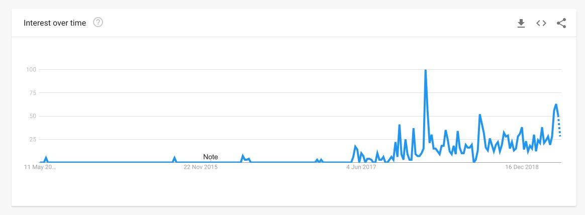
AutoML algorithms are reaching really good rankings in data science competitions (see this article)
But what is AutoML ? How does it work? And mainly, how can you implement an AutoML in Python?
What is AutoML?
AutoML is a framework whose role is to optimize the machine learning workflow, which includes automatic training and tuning of many models within a user-specified time-limit.
The idea is to fasten the work of the Data Scientist when it comes to model selection and parameter tuning. On the other hand, the user simply inputs the training data, eventually some validation data, and a time limit.
AutoML will automatically try several models, choose the best performing models, tune the parameters of the leader models, try to stack them…
AutoML outputs a leaderboard of algorithms, and you can select the best performing algorithm given several criteria that are measured (MSE, RMSE, log loss, Auc…).
Why and when should you use AutoML?
Building models and tuning the hyperparameters is a long process for any data scientist. The search space for the optimal parameters is enormous, and this is only for 1 chosen model.
AutoML can be highly parallelized, so bear in mind that a couple of GPUs will help.
AutoML can be used to :
- Assess the feature importance
- Try a lot of models and parameters as a first guess
Once a model and a set of parameters have been identified, you have 2 options :
- either the model is good enough and satisfies your criteria
- or you can use the selected set of model + parameters as a starting point for a GridSearch or Bayesian HyperOpt
How does AutoML work?
AutoML does not use a GIANT double for-loop to test every model and every parameter. It’s much smarter than that. It uses Reinforcement Learning.
A controller neural net can propose a “child” model architecture, which can then be trained and evaluated for quality on a particular task. That feedback is then used to inform the controller how to improve its proposals for the next round.
Eventually, the controller learns to assign a high probability to areas of architecture space that achieve better accuracy on a held-out validation dataset, and low probability to areas of architecture space that score poorly.
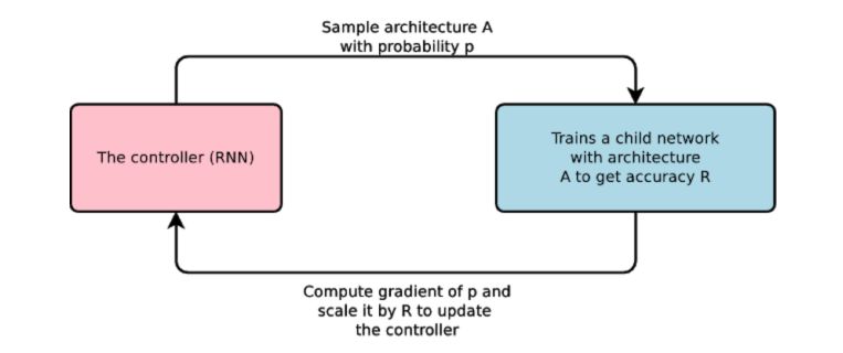
To make the controller a little more complex, it uses anchor points, and set-selection attention to form skip connections.
At that point, you might think that AutoML frameworks are extremely long to run. In AutoML, each gradient update to the controller parameters θ corresponds to training one child network to convergence.
You’re right, training a single child network can take hours. For this reason, according to Google’s Blog, AutoML uses distributed training and asynchronous parameter updates to speed up the learning process of the controller. It uses a parameter-server scheme where we have a parameter server of S shards, that store the shared parameters for K controller replicas. Each controller replica samples m different child architectures that are trained in parallel. The controller then collects gradients according to the results of that minibatch of m architectures at convergence and sends them to the parameter server to update the weights across all controller replicas.
Example in Python
Several companies are currently AutoML pipelines. Among them, Google and h2o. In this example, we’ll use h2o’s solution. I suggest you run this in Google Colab using GPU’s, but you can also run it locally.
Start by importing the necessary packages :
!pip install requests
!pip install tabulate
!pip install "colorama>=0.3.8"
!pip install future
!pip install -f http://h2o-release.s3.amazonaws.com/h2o/latest_stable_Py.html h2o
The Data
We’ll use the Credit Card Fraud detection, a famous Kaggle dataset that can be found here.
The dataset contains transactions made by credit cards in September 2013 by European cardholders. This dataset presents transactions that occurred in two days, where we have 492 frauds out of 284,807 transactions. The dataset is highly unbalanced, the positive class (frauds) account for 0.172% of all transactions.
It contains only numerical input variables which are the result of a PCA transformation. Unfortunately, due to confidentiality issues, the original features are not provided. Features V1, V2, … V28 are the principal components obtained with PCA, the only features which have not been transformed with PCA are ‘Time’ and ‘Amount’. Feature ‘Time’ contains the seconds elapsed between each transaction and the first transaction in the dataset. The feature ‘Amount’ is the transaction Amount, this feature can be used for example-dependant cost-sensitive learning. Feature ‘Class’ is the response variable and it takes value 1 in case of fraud and 0 otherwise.
### General
import numpy as np
import pandas as pd
import matplotlib.pyplot as plt
df = pd.read_csv('creditcard.csv')
df.head()

If you explore the data, you’ll notice that only 0.17% of the transactions are fraudulent. We’ll use the F1-Score metric, a harmonic mean between the precision and the recall.
To understand the nature of the fraudulant transactions, simply plot the following graph :
plt.figure(figsize=(12,8))
plt.scatter(df[df.Class == 0].Time, df[df.Class == 0].Amount, c='green', alpha=0.4, label="Not Fraud")
plt.scatter(df[df.Class == 1].Time, df[df.Class == 1].Amount, c='red', label="Fraud")
plt.title("Amount of the transaction over time")
plt.legend()
plt.show()
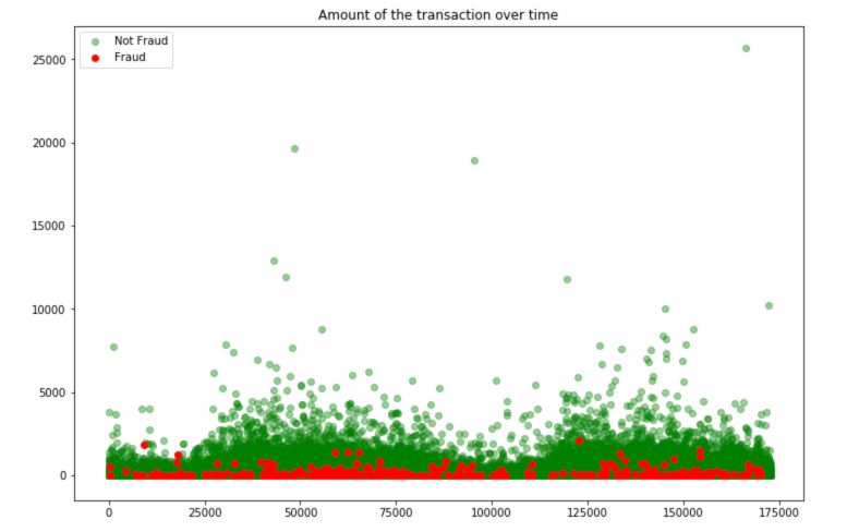
Fraudulent transactions have a limited amount. We can guess that these transactions must remain “unseen” and not attracting too much attention.
h2o AutoML
Now, let’s import h2o AutoML :
### h2o AutoML
import h2o
from h2o.estimators.gbm import H2OGradientBoostingEstimator
from h2o.automl import H2OAutoML
The, initialize the h2o session :
# Initialize
h2o.init()
If you’re running this locally, you should see something like this :
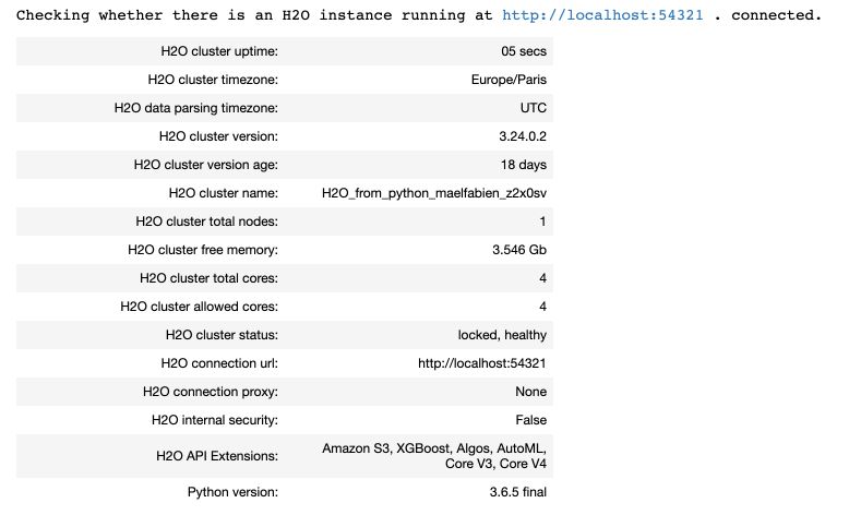
If you follow the local link to the instance, you can access the h2o Flow :
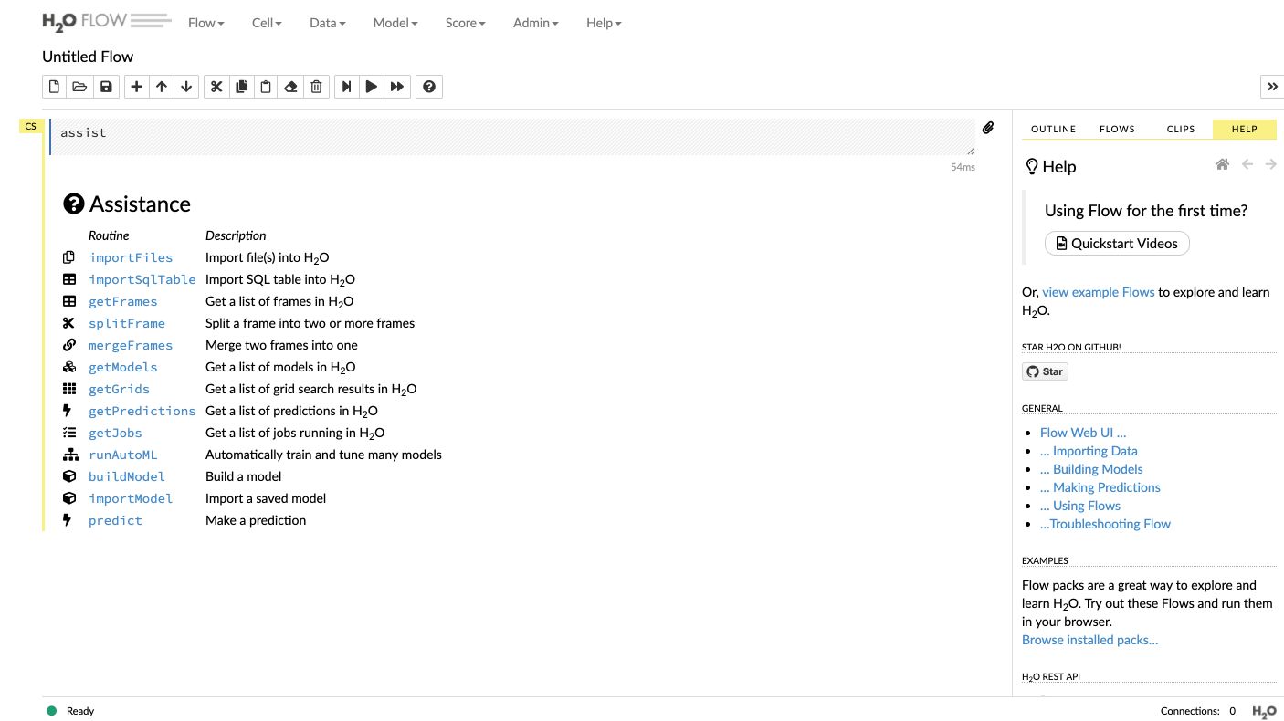
I’ll further explore Flow in another article, but Flow aims to do the same thing with a visual interface. In h2o, you need to import the dataset as an h2o object, and use built-in functions to split the data frame :
# Load the data
df = h2o.import_file("/Users/maelfabien/Desktop/LocalDB/CreditCard/creditcard.csv")

d = df.split_frame(ratios = [0.8], seed = 1234)
df_train = d[0] # using 80% for training
df_test = d[1] #rest 20% for testing
We then define a list of the columns we’ll use as predictors :
# Predictor columns
predictors = list(df.columns)
predictors.remove('Time')
predictors.remove('Class')
As you might have guessed, we’re facing a binary classification problem here. The default case is regression in AutoML. To “cast” a column type to integer, use this :
# Cast binary
df_train['Class'] = df_train['Class'].asfactor()
We are now ready to define the model and train it. We specify the maximal number of models to test, and the overall maximal runtime in seconds.
aml = H2OAutoML(max_models = 50, seed = 1, max_runtime_secs=21000)
aml.train(x = predictors, y = 'Class', training_frame = df_train, validation_frame = df_test)
By default, the maximal runtime is 1 hour. Your model will be training for 21’000 seconds now (I left it to train overnight). Now, let’s display all the models that have been tested and their performance :
print(aml.leaderboard)
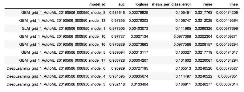
The leaderboard is established using Cross Validation, which more or less guarantees that the top performing models are indeed consistently performing well.
To display only the best model, use print(aml.leader).
We can now make a prediction using the leader model, simply using:
aml.leader.predict(new_data)
We can then save the best model :
h2o.save_model(aml.leader, path = "./model_credit_card")
Once your work is over, shut down the session :
h2o.shutdown()
In this simple example, h2o outperformed the tuning I manually did.
Conclusion : I hope this article on AutoML was interesting. It’s a really hot topic, and I do expect large improvements to be made over the next years in this field.
Sources :
