
Xception is a deep convolutional neural network architecture that involves Depthwise Separable Convolutions. It was developed by Google researchers. Google presented an interpretation of Inception modules in convolutional neural networks as being an intermediate step in-between regular convolution and the depthwise separable convolution operation (a depthwise convolution followed by a pointwise convolution). In this light, a depthwise separable convolution can be understood as an Inception module with a maximally large number of towers. This observation leads them to propose a novel deep convolutional neural network architecture inspired by Inception, where Inception modules have been replaced with depthwise separable convolutions.
The original paper can be found here.
I. What is an XCeption network?
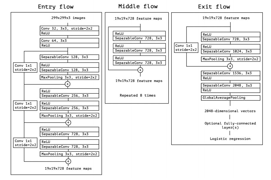
What does it look like?
The data first goes through the entry flow, then through the middle flow which is repeated eight times, and finally through the exit flow. Note that all Convolution and SeparableConvolution layers are followed by batch normalization.
Xception architecture has overperformed VGG-16, ResNet and Inception V3 in most classical classification challenges.
How does XCeption work?
XCeption is an efficient architecture that relies on two main points :
- Depthwise Separable Convolution
- Shortcuts between Convolution blocks as in ResNet
Depthwise Separable Convolution
Depthwise Separable Convolutions are alternatives to classical convolutions that are supposed to be much more efficient in terms of computation time.
The limits of convolutions
First of all, let’s take a look at convolutions. Convolution is a really expensive operation. Let’s illustrate this :

The input image has a certain number of channels C, say 3 for a color image. It also has a certain dimension A, say 100 * 100. We apply on it a convolution filter of size d*d, say 3*3. Here is the convolution process illustrated :
Now, how many operations does that make?
Well, for 1 Kernel, that is :
\[K^2 \times d^2 \times C\]Where K is the resulting dimension after convolution, which depends on the padding applied (e.g padding “same” would mean A = K).
Therefore, for N Kernels (depth of the convolution) :
\[K^2 \times d^2 \times C \times N\]To overcome the cost of such operations, depthwise separable convolutions have been introduced. They are themselves divided into 2 main steps :
- Depthwise Convolution
- Pointwise Convolution
The Depthwise Convolution
Depthwise Convolution is a first step in which instead of applying convolution of size \(d \times d \times C\), we apply a convolution of size \(d \times d \times 1\). In other words, we don’t make the convolution computation over all the channels, but only 1 by 1.
Here is an illustration of the Depthwise convolution process :
This creates a first volume that has size \(K \times K \times C\), and not \(K \times K \times N\) as before. Indeed, so far, we only made the convolution operation for 1 kernel /filter of the convolution, not for \(N\) of them. This leads us to our second step.
Pointwise Convolution
Pointwise convolution operates a classical convolution, with size \(1 \times 1 \times N\) over the \(K \times K \times C\) volume. This allows creating a volume of shape \(K \times K \times N\), as previously.
Here is an illustration of the Pointwise Convolution :
Alright, this whole thing looks fancy, but did we reduce the number of operations? Yes we did, by a factor proportional to \(\frac {1} {N}\) (this can be quite easily shown).
Implementation of the XCeption
XCeption offers an architecture that is made of Depthwise Separable Convolution blocks + Maxpooling, all linked with shortcuts as in ResNet implementations.
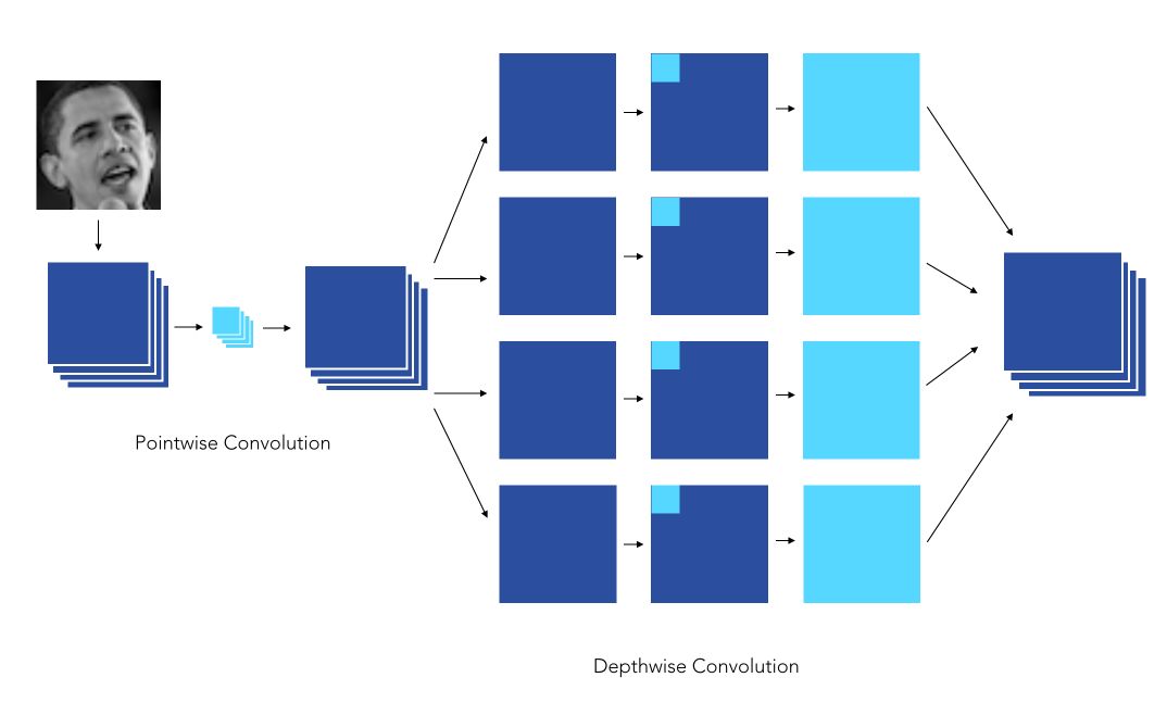
The specificity of XCeption is that the Depthwise Convolution is not followed by a Pointwise Convolution, but the order is reversed, as in this example :
II. In Keras
Let’s import the required packages :
import tensorflow as tf
import tensorflow.keras

from tensorflow.keras import models, layers
from tensorflow.keras.models import Model, model_from_json, Sequential

from tensorflow.keras.preprocessing.image import ImageDataGenerator, array_to_img, img_to_array, load_img
from tensorflow.keras.callbacks import TensorBoard
from tensorflow.keras.layers import Dense, Dropout, Activation, Flatten, Conv2D, MaxPooling2D, SeparableConv2D, UpSampling2D, BatchNormalization, Input, GlobalAveragePooling2D

from tensorflow.keras.regularizers import l2
from tensorflow.keras.optimizers import SGD, RMSprop
from tensorflow.keras.utils import to_categorical
from keras.utils.vis_utils import plot_model
Import our data. I’m working on the Facial Emotion Recognition 2013 challenge from Kaggle. The path links to my local storage folder :
X_train = np.load(path + "X_train.npy")
X_test = np.load(path + "X_test.npy")
y_train = np.load(path + "y_train.npy")
y_test = np.load(path + "y_test.npy")
Now, let’s build the Entry Flow!
def entry_flow(inputs) :

    x = Conv2D(32, 3, strides = 2, padding='same')(inputs)
    x = BatchNormalization()(x)
    x = Activation('relu')(x)

    x = Conv2D(64,3,padding='same')(x)
    x = BatchNormalization()(x)
    x = Activation('relu')(x)

    previous_block_activation = x

    for size in [128, 256, 728] :

        x = Activation('relu')(x)
        x = SeparableConv2D(size, 3, padding='same')(x)
        x = BatchNormalization()(x)

        x = Activation('relu')(x)
        x = SeparableConv2D(size, 3, padding='same')(x)
        x = BatchNormalization()(x)

        x = MaxPooling2D(3, strides=2, padding='same')(x)

        residual = Conv2D(size, 1, strides=2, padding='same')(previous_block_activation)

        x = tensorflow.keras.layers.Add()([x, residual])
        previous_block_activation = x

    return x
Add the Middle Flow :
def middle_flow(x, num_blocks=8) :

    previous_block_activation = x

    for _ in range(num_blocks) :

        x = Activation('relu')(x)
        x = SeparableConv2D(728, 3, padding='same')(x)
        x = BatchNormalization()(x)

        x = Activation('relu')(x)
        x = SeparableConv2D(728, 3, padding='same')(x)
        x = BatchNormalization()(x)

        x = Activation('relu')(x)
        x = SeparableConv2D(728, 3, padding='same')(x)
        x = BatchNormalization()(x)

        x = tensorflow.keras.layers.Add()([x, previous_block_activation])
        previous_block_activation = x

    return x
And finally the Exit Flow :
def exit_flow(x) :

    previous_block_activation = x

    x = Activation('relu')(x)
    x = SeparableConv2D(728, 3, padding='same')(x)
    x = BatchNormalization()(x)

    x = Activation('relu')(x)
    x = SeparableConv2D(1024, 3, padding='same')(x)
    x = BatchNormalization()(x)

    x = MaxPooling2D(3, strides=2, padding='same')(x)

    residual = Conv2D(1024, 1, strides=2, padding='same')(previous_block_activation)
    x = tensorflow.keras.layers.Add()([x, residual])

    x = Activation('relu')(x)
    x = SeparableConv2D(728, 3, padding='same')(x)
    x = BatchNormalization()(x)

    x = Activation('relu')(x)
    x = SeparableConv2D(1024, 3, padding='same')(x)
    x = BatchNormalization()(x)

    x = GlobalAveragePooling2D()(x)
    x = Dense(1, activation='linear')(x)

    return x
This architecture leads to a limited number of trainable parameters compared to an equivalent depth in classical convolutions.
We can build the model :
inputs = Input(shape=(shape_x, shape_y, 1))
outputs = exit_flow(middle_flow(entry_flow(inputs)))
xception = Model(inputs, outputs)
If you would like to visualize the model architecture, use plot_model :
plot_model(xception, to_file='model.png', show_shapes=True, show_layer_names=True)

We are finally ready to compile the model.
xception.compile(optimizer='adam', loss='categorical_crossentropy', metrics=['accuracy'])

batch_size = 128
epochs = 150
And run it!
history = xception.fit(X_train, y_train, epochs=150, batch_size=64, validation_data=(X_test, y_test))
The Github repository of this article can be found here.
Conclusion : Xception models remain expensive to train, but are pretty good improvements compared to Inception. Transfer learning brings part of the solution when it comes to adapting such algorithms to your specific task.