
In this short article, we are going to cover the concepts of the main regularization techniques in deep learning, and other techniques to prevent overfitting.
Overfitting
Overfitting can be graphically observed when your training accuracy keeps increasing while your validation/test accuracy does not increase anymore.
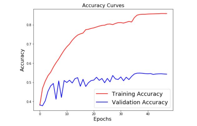
If we only focus on the training accuracy, we might be tempted to select the model that heads the best accuracy in terms of training accuracy. This is, however, a dangerous approach since the validation accuracy should be our control metric.
One of the major challenges of deep learning is avoiding overfitting. Therefore, regularization offers a range of techniques to limit overfitting. They include :
- Train-Validation-Test Split
- Class Imbalance
- Drop-out
- Data Augmentation
- Early stopping
- L1 or L2 Regularization
- Learning Rate Reduction on Plateau
- Save the best model
We’ll create a small neural network using Keras Functional API to illustrate this concept.
import tensorflow.keras
from tensorflow.keras.preprocessing.image import ImageDataGenerator, array_to_img, img_to_array, load_img
from tensorflow.keras.callbacks import TensorBoard
from tensorflow.keras.models import Sequential
from tensorflow.keras.layers import Dense, Dropout, Activation, Flatten, Conv2D, MaxPooling2D,
from tensorflow.keras.regularizers import l2
We’ll consider a simple Computer Vision algorithm that could typically suit the MNIST dataset.
input_img = Input(shape=(28, 28, 1))
Train-Validation-Test Split
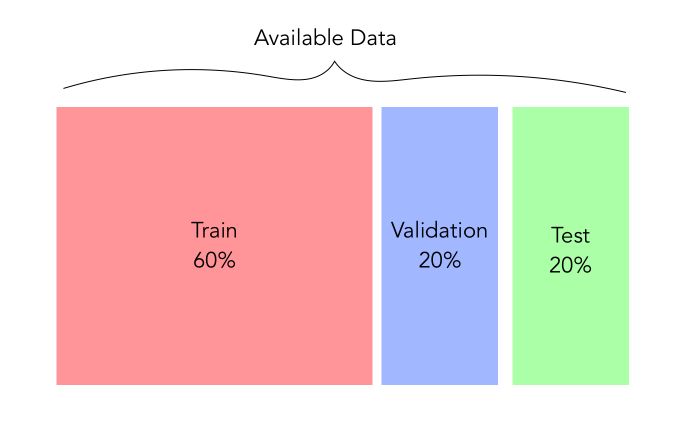
The first reflex when you face a sufficient amount of data and are about to apply deep learning techniques would be to create 3 sets :
- a train set used to train the model.
- a validation set used to select the hyperparameters of the model and control for overfitting
- a test set used to test the final accuracy of our model
For example, here is a typical split you could be using :
In Keras, once you have built the model, simply specify the validation data this way :
model = model.fit(X_train, y_train, epochs = epochs, batch_size=batch_size, validation_data=(X_val, y_val))
pred = model.predict(X_test)
print(accuracy_score(pred, y_test)
There is also a cool feature in Keras to make the split automatically and therefore create a validation set :
model = model.fit(X_train, y_train, epochs = epochs, batch_size=batch_size, validation_split=0.2)
pred = model.predict(X_test)
print(accuracy_score(pred, y_test)
Once the right model has been chosen and tuned, you should train in on the whole amount of data available. If you don’t have a sufficient amount of data, you can make the model choice based on :
- Grid Search or HyperOpt
- K-Fold Cross-Validation
Class Imbalance
Sometimes, you might face a large class imbalance. This is typically the case for fraud detection, emotion recognition…
In such case, if the imbalance is large, as below if data collection is not possible, you should maybe think of helping the network a little bit with manually specified class weights.
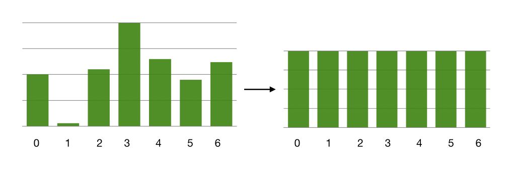
Class weights directly affect the loss function, by modifying the amount of data of each class sent in each batch. Therefore, we have an equivalent amount of data from each class sent in each batch. This, however, requires that the amount of data in the minor class remains sufficiently important so that there is no overfitting on 200 examples being reused all the time for example.
Here is how you can implement class weight in Keras :
class_weight = {
    0:1/sum(y_train[:,0]),
    1:1/sum(y_train[:,1]),
    2:1/sum(y_train[:,2]),
    3:1/sum(y_train[:,3]),
    4:1/sum(y_train[:,4]),
    5:1/sum(y_train[:,5]),
    6:1/sum(y_train[:,6])
}
And when fitting your model :
```python
model = model.fit(X_train, y_train, epochs = epochs, batch_size=batch_size, validation_split=0.2, class_weight = class_weight)
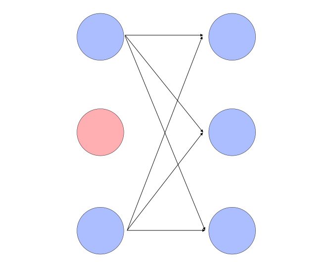
Drop-out
The drop-out technique allows us for each neuron, during training, to randomly turn-off a connection with a given probability. This prevents co-adaptation between units. In Keras, the dropout is simply implemented this way :
x = Conv2D(64, (3, 3), padding='same')(input_img)
x = BatchNormalization()(x)
x = Activation('relu')(x)
x = Dropout(0.25)(x)
Data Augmentation
Data augmentation is a popular way in image classification to prevent overfitting. The concept is to simply apply slight transformations on the input images (shift, scale…) to artificially increase the number of images. For example, in Keras :
datagen = ImageDataGenerator(zoomrange=0.2,# randomly zoom into images
    rotationrange=10,# randomly rotate images
    widthshiftrange=0.1,# randomly shift images horizontally
    heightshiftrange=0.1,# randomly shift images vertically
    horizontalflip=True,# randomly flip images
    verticalflip=False)# randomly flip images
The transformations would typically look like this :

Then, when fitting your model :
model.fit_generator(
    datagen.flow(X_train, y_train, batch_size=batch_size),
    steps_per_epoch=int(np.ceil(X_train.shape[0] / float(batch_size))),
    epochs = epochs,
    class_weight = class_weight,
    validation_data=(X_test, y_test))
Early stopping
Early Stopping is a way to stop the learning process when you notice that a given criterion does not change over a series of epochs. For example, if we want the validation accuracy to increase, and the algorithm to stop if it does not increase for 10 periods, here is how we would implement this in Keras :
earlyStopping = EarlyStopping(monitor='val_acc', patience=10, verbose=0, mode='max')
Then, when fitting the model :
model.fit_generator(
    datagen.flow(X_train, y_train, batch_size=batch_size),
    steps_per_epoch=int(np.ceil(X_train.shape[0] / float(batch_size))),
    epochs = epochs,
    callbacks=[earlyStopping],
    class_weight = class_weight,
    validation_data=(X_test, y_test))
Regularization
Regularization techniques (L2 to force small parameters, L1 to set small parameters to 0), are easy to implement and can help your network. The L2-regularization penalizes large coefficients and therefore avoids overfitting.
For example, on the layer of your network, add :
x = Dense(nb_classes, activation='softmax', activity_regularizer=l2(0.001))(x)
Learning Rate Reduction on Plateau
This technique is quite interesting and can help your network. Even if you have an “Adam” or “RMSProp” optimizer, your network might get stuck at some point on a plateau. In such a case, it might be useful to reduce the learning rate and try to get those extra percent of accuracy. Indeed, a learning rate a bit too large might simply mean that you overshoot the minimum and are kind of stuck close to a minimal point.
In Keras, here’s how to do it :
reduce_lr_acc = ReduceLROnPlateau(monitor='val_acc', factor=0.1, patience=7, verbose=1, min_delta=1e-4, mode='max')
And when you fit the model :
model.fit_generator(
    datagen.flow(X_train, y_train, batch_size=batch_size),
    steps_per_epoch=int(np.ceil(X_train.shape[0] / float(batch_size))),
    epochs = epochs,
    callbacks=[earlyStopping, reduce_lr_acc],
    class_weight = class_weight,
    validation_data=(X_test, y_test))
Here is for example something that happened to me the day I wrote the article :
Epoch 32/50
28709/28709 [==============================] - 89s 3ms/sample - loss: 0.1260 - acc: 0.8092 - val_loss: 3.7332 - val_acc: 0.5082
Epoch 33/50
28709/28709 [==============================] - 88s 3ms/sample - loss: 0.1175 - acc: 0.8134 - val_loss: 3.7183 - val_acc: 0.5269
Epoch 34/50
28709/28709 [==============================] - 89s 3ms/sample - loss: 0.1080 - acc: 0.8178 - val_loss: 3.8838 - val_acc: 0.5143
Epoch 35/50
28704/28709 [============================>.] - ETA: 0s - loss: 0.1119 - acc: 0.8150
Epoch 00035: ReduceLROnPlateau reducing learning rate to 0.00010000000474974513.
28709/28709 [==============================] - 103s 4ms/sample - loss: 0.1120 - acc: 0.8149 - val_loss: 3.7373 - val_acc: 0.5311
Epoch 36/50
28709/28709 [==============================] - 92s 3ms/sample - loss: 0.0498 - acc: 0.8374 - val_loss: 3.7629 - val_acc: 0.5436
Epoch 37/50
28709/28709 [==============================] - 91s 3ms/sample - loss: 0.0182 - acc: 0.8505 - val_loss: 4.0153 - val_acc: 0.5478
Epoch 38/50
28709/28709 [==============================] - 91s 3ms/sample - loss: 0.0119 - acc: 0.8539 - val_loss: 4.1941 - val_acc: 0.5483
Once the learning rate reduced, the validation accuracy greatly improved.
Save the best model
At a given epoch, you might encounter a model that reaches a really good accuracy compared to other epochs. But how can you save this model precisely? Using checkpoints!
mcp_save = ModelCheckpoint('path-to-model/model.hdf5', save_best_only=True, monitor='val_acc', mode='max')
Set the option save_best_only to True and the checkpoint will only save the weights of the model at the next iteration if the validation accuracy is maximized. You can select any criteria, such as “Min val_loss” for example.
*Conclusion *: I hope this quick article gave you some idea on how to prevent overfitting on your next neural network in Keras! Don’t hesitate to drop a comment.