
Now we have covered the concept on Perceptron, it is time to move on to the so-called Multilayer Perceptron (MLP)
Definition
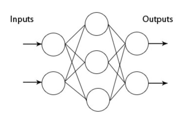
A multilayer perceptron is a feedforward artificial neural network (ANN), made of an input layer, one or several hidden layers, and an output layer.
The phase of “learning” for a multilayer perceptron is reduced to determining for each relationship between each neuron of two consecutive layers :
- the weights \(w_i\)
- the biases \(b_i\)
One major difference with the Rosenblatt perceptron is that the structure, due to the multiplicity of (hidden) layers, is no longer linear and allows us to model more complex data structures.
Maximum Likelihood Estimate (MLE)
Such values are determined using the concept of maximum likelihood estimations (MLE). The maximum likelihood estimate \(\hat{\theta}^{MLE}\) determines the parameters which maximize the probability of observing \(\theta\) For classification problems, the maximum likelihood optimization can be expressed as follows :
\[\hat{\theta}^{MLE} = {argmax}_\theta P(Y|X, \theta)\]where \(\theta =[W^{(l)}, b^{(l)}]\). We suppose that we have \(n\) training samples, and that each sample has the same number of classes \(k\).
Assuming that the \(Y_n\) are identically and independently distributed (iid), which will in most cases be the assumption, we know that :
\[Y_n ~^{iid} P(Y | X, \theta)\]Therefore :
\[\hat{\theta}^{MLE} = {argmax}_\theta \prod P(Y_n|X_n, \theta)\]In the context of classification, labels will follow a Bernouilli distribution. We can state that :
\[\hat{\theta}^{MLE} = {argmax}_\theta \prod_n \prod_k P(Y_n=k|X_{n}, \theta)^{t_{n,k}}\]where \(t_{n,k}\) is a one-hot encoded version of our labels \(Y\). As a sample always belong to a class, we know that :
\[\sum_k P(Y_n=k|X_{n}, \theta) = 1\]We can focus on the log-likelihood to make the computations easier and work with sums instead of products :
\[\hat{\theta}^{MLE} = {argmax}_\theta \sum_n \sum_k t_{n,k} log(P(Y_n=k|X_{n}, \theta))\]When dealing with classification problems, we want to minimize the classification error, which is expressed as the negative log-likelihood (NLL) :
\[NLL(\theta) = -l(\theta) = - \sum_n \sum_k t_{n,k} log(P(Y_n=k|X_{n}, \theta))\]For a single sample, the measure is called the cross-entropy loss :
\[NLL(\theta) = - \sum_k t_{n,k} log(P(Y_n=k|X_{n}, \theta))\]We can indeed prove the equivalence between minimizing the loss and maximizing the likelihood. We need to find (\theta^{MLE}) that minimizes this loss. Note that the MLE produces an unbiaised estimator, i.e \(E(\hat{\theta}^{MLE}) = \theta^*\)
As we do not have access to the potential entire data set, but to a sample only, we minimize the cost (the sum of the losses) given the concept of Empirical Risk Minimization (ERM).
Activation functions
Activation functions are essential to build a multilayer perceptron. They bring non-linearity in the structure of MLPs. There are several activation functions that can be used. The activation functions can vary depending on the layer we consider. The most popular activation functions are the following :
- sigmoid : \({\sigma(z)} = \frac {1}{1 + e^{-z}}\)
- hyperbolic tangent : \({g(z)} = \frac {e^{z} - e^{-z}}{e^{z} + e^{-z}}\)
- rectified linear unit (ReLU) : \({g(z)} = max(0,z)\)
- leaky ReLU : \({g(z)} = max(0.01z,z)\)
- parametric ReLU (PReLU) : \({g(z)} = max(\alpha z,z)\)
- softplus function : \({g(z)} = log(1 + e^z)\)
In practice, for our face emotion recognition problem, we tend to use the ReLU activation function. Indeed, the ReLU is not subject to the vanishing gradient problem. It has issues dealing with negative inputs, but since our input takes the form of arrays describing colors of pixels, we only have positive inputs.
These activations functions are commonly used on the hidden layers. For the output layer, we commonly use another activation function called the \(softmax\) activation. The \(softmax\) allows a transformation of the output layer into probabilities for each class. For classification purposes, we then only select the maximal probability as the class computed.
\[{g(z)_j} = \frac {e^{z_j}}{\sum_k e^{z_k}}\]Gradient descent
There are two ways to solve this minimization problem :
- using traditional calculus, but this typically produces long and un-intuitive equations
- using stochastic gradient descent
Stochastic gradient descent offers a two-step gradient descent (forward propagation, and backpropagation) that allows us to approach the solution in a computationally efficient way. The stochastic gradient descent takes each observation individually and computes a gradient descent. Then, the overall gradient is averaged. On the other hand, the batch gradient descent needs to wait until the optimal gradient has been computed on all training observations.
The forward propagation consists of applying a set of weights, bias and activation functions to an input layer to compute the output. Then, while learning from our classification errors, we update the weights by moving backward. This is the backpropagation.
We won’t cover the details of the back propagation, but for the intuition, it is enough to state that the concept of back propagation is a simple application of the chain rule that allows :
\[\frac {\partial}{\partial t} f(x(t)) = \frac {\partial f} {\partial x} \frac {\partial x} {\partial t}\]In practice, the stochastic gradient descent is however rarely used. Some improved alternatives are preferred, including :
- Mini batch gradient descent, which performs an update for every mini-batch of (n) training examples, but cannot guarantee good convergence due to the choice of the learning rate
- Momentum, a method that helps accelerate stochastic gradient descent in the relevant direction and dampens oscillations by adding a fraction of the past time step to the current one
- Adaptive Moment Estimation (Adam), that computes adaptive learning rates for each parameter.
Implementation in Tensorflow
def init_weights_and_biases(shape, stddev=0.1, seed_in=None):
"""
This function should return Tensorflow Variables containing the initialized weights and biases of the network,
using a normal distribution for the initialization, with stddev of the normal as an input argument

Parameters
----------
shape : tuple, (n_input_features,n_hidden_1, n_hidden_2,n_classes)
sizes necessary for defining the weights and biases

Returns
-------
w1, b1, w2, b2, w3, b3 : Tensorflow Variables
initialized weights and biases, with correct shapes
"""

w1 = tf.Variable(tf.random_normal([shape[0], shape[1]], stddev=stddev), name='w1')
b1 = tf.Variable(tf.random_normal([shape[1]]), name='b1')

w2 = tf.Variable(tf.random_normal([shape[1], shape[2]], stddev=stddev), name='w2')
b2 = tf.Variable(tf.random_normal([shape[2]]), name='b2')

w3 = tf.Variable(tf.random_normal([shape[2], shape[3]], stddev=stddev), name='w3')
b3 = tf.Variable(tf.random_normal([shape[3]]), name='b3')

return w1, b1, w2, b2, w3, b3

def forward_prop_multi_layer(X, w1, b1, w2, b2, w3, b3):
"""
This function should define the network architecture, explained above

Parameters
----------
X: input to the network
w1, w2, w3: Tensorflow Variables
network weights
b1, b2, b3: Tensorflow Variables
network biases

Returns
-------
Y_pred :
the output layer of the network, the classification prediction
"""

hidden_1 = tf.nn.sigmoid(tf.add(tf.matmul(X,w1), b1))
hidden_2 = tf.nn.sigmoid(tf.add(tf.matmul(hidden_1,w2), b2))
Y_pred = tf.nn.softmax(tf.add(tf.matmul(hidden_2,w3), b3))

return Y_pred
RANDOM_SEED = 52
tf.set_random_seed(RANDOM_SEED)

# Network Parameters
n_hidden_1 = 256 # 1st layer number of neurons
n_hidden_2 = 256 # 2nd layer number of neurons
n_input = X_train.shape[1]
n_classes = Y_train.shape[1] # MNIST total classes (0-9 digits)

# tf Graph input
X_input = tf.placeholder("float", [None, n_input])
Y_true = tf.placeholder("float", [None, n_classes])

# Weight and bias initialisations
stddev = 0.1
w1,b1,w2,b2,w3,b3 = init_weights_and_biases([n_input, n_hidden_1, n_hidden_2,n_classes], stddev=0.1, seed_in=RANDOM_SEED)

# Construct model
Y_pred = forward_prop_multi_layer(X_input,w1,b1,w2,b2,w3,b3)

# Define loss and optimizer
cross_entropy = -tf.reduce_sum(Y_true * tf.log(Y_pred),axis=1)

loss = tf.reduce_mean(cross_entropy)
acc = accuracy(Y_pred, Y_true)

learning_rate = 0.001
optimizer = tf.train.AdamOptimizer(learning_rate=learning_rate)
training_variables = optimizer.minimize(loss)

# Parameters
n_epochs = 20
train_accuracy = []
test_accuracy = []
batch_size = 100
display_step = 1
n_batches = int(np.ceil(X_train.shape[0]/batch_size))

with tf.Session() as sess:
# Initializing the variables
init = tf.global_variables_initializer()
sess.run(init)

for epoch in range(n_epochs):
# Loop over all batches
for batch_idx in range(n_batches):
#get the next batch in the MNIST dataset and carry out training
#BEGIN STUDENT CODE
batch_x = X_train[batch_idx * batch_size : (batch_idx + 1) * batch_size]
batch_y = Y_train[batch_idx * batch_size : (batch_idx + 1) * batch_size]
sess.run(training_variables, feed_dict={X_input:batch_x, Y_true:batch_y})

#END STUDENT CODE
# calculate accuracy for this epoch
train_accuracy.append(sess.run(acc, feed_dict={X_input: X_train,Y_true:Y_train}))
test_accuracy.append(sess.run(acc,  feed_dict={X_input: X_test,Y_true:Y_test}))

print(".", end='')
print("Training finished")

#plot the accuracy
plot_accuracy(train_accuracy,test_accuracy)
The Github repository of this article can be found here.
Conclusion: The MLP is the base model for several other deep learning algorithms (CNN, RNN…). These algorithms typically find applications in the field of natural language processing, computer vision, signal processing… We will get more into details into further articles!