This series of articles provides a summary of the course : “Introduction to Deep Learning with PyTorch” on Udacity.

The Perceptron : Key concepts

The perceptron can be seen as a mapping of inputs into neurons. Each input is represented as a neuron :

(I wrote an article on the topic if you’d like to learn more on this topic)

We attach to each input a weight ( \(w_i\)) and notice how we add an input of value 1 with a weight of \(- \theta\). This is called bias. What we are doing is instead of having only the inputs and the weight and compare them to a threshold, we also learn the threshold as a weight for a standard input of value 1.

The inputs can be seen as neurons and will be called the input layer. Altogether, these neurons and the function (which we’ll cover in a minute) form a perceptron.

How do we make classification using a perceptron then?

\(y = 1\) if \(\sum_i w_i x_i ≥ 0\), else \(y = 0\)

The classification that checks of the output is greater than 0 is called a step function.

Logical operators

Perceptron can be used to represent logical operators. For example, one can represent the perceptron as an “AND” operator.

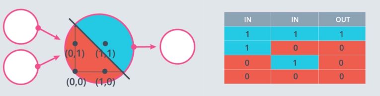
A simple “AND” perceptron can be built in the following way :

weight1 = 1.0
weight2 = 1
bias = -1.2

linear_combination = weight1 * input_0 + weight2 * input_1 + bias
output = int(linear_combination >= 0)

Where input_0 and input_1 represent the two feature inputs. We are shifting the bias by 1.2 to isolate the positive case where both inputs are 1.

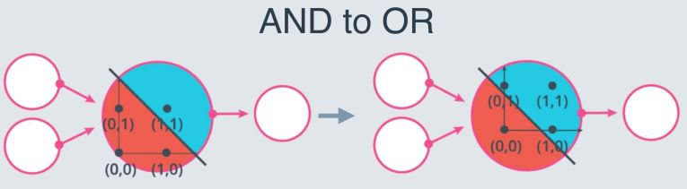
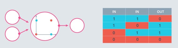
However, solving the XOR problem is impossible :

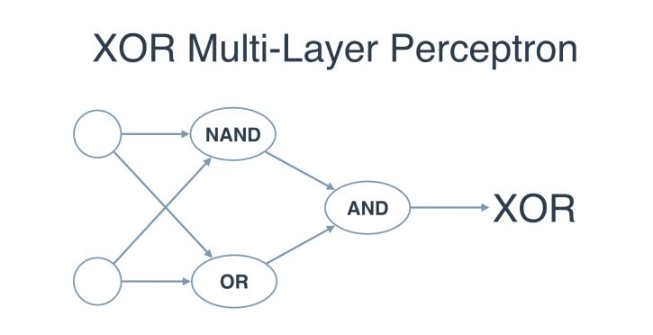
This is why Multi-layer perceptrons were introduced. In Multi-layer perceptrons, we can build XOR as a combination of logical operators perceptrons :

Finding the weights

How do we identify the right weights that allow the best split ?

Suppose we have an initial equation with random weights set as : \(3 X_1 + 4 X_2 - 10 = 0\)

If the point (4,5) is misclassified and should belong to the class -1, and we have a learning rate of 0.1, what we’ll do is update the weights the following way :

\[3 - 0.1 * 4 = 2.6\] \[4 - 0.1 * 5 = 3.5\] \[-10 - 0.1 * 1 = -10.1\]

We are slowly shifting the line towards the point that was misclassified. the new equation is therefore :

\[2.6 X_1 + 3.5 X_2 - 10.1 = 0\]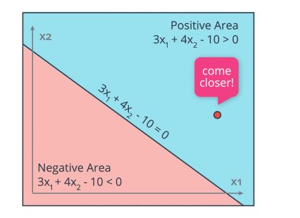

If another point is misclassified and should belong to the positive class, we’ll apply the same process except we’ll add weights.

To summarize, the pseudo-code for the Perceptron is the following :

Initialize random weights \(w_1, ..., w_n, b\)
For every misclassified point \(X_1, ..., X_n\) :
- If the prediction is 0 :
  - For \(i = 1...n\) :
    - \[W_i = W_i + \alpha X_i\]
  - \[b_i = b_i + \alpha\]
- If the prediction is 1 :
  - For \(i = 1...n\) :
    - \[W_i = W_i - \alpha X_i\]
  - \[b_i = b_i - \alpha\]

Implementation in Python

We can quite simply implement a Perceptron in Python :

import numpy as np

def stepFunction(t):
    if t >= 0:
        return 1
    return 0

def prediction(X, W, b):
    return stepFunction((np.matmul(X,W)+b)[0])

def perceptronStep(X, y, W, b, learn_rate = 0.01):
    # Fill in code
    for i in range(len(y)):
        y_hat = prediction(X[i],W,b)
        if y[i] - y_hat == 1:
            W[0] += learn_rate * X[i][0]
            W[1] += learn_rate * X[i][1]
            b += learn_rate
        elif y[i] - y_hat == -1:
            W[0] -= learn_rate * X[i][0]
            W[1] -= learn_rate * X[i][1]
            b -= learn_rate
    return W, b
    
def trainPerceptronAlgorithm(X, y, learn_rate = 0.01, num_epochs = 25):
    x_min, x_max = min(X.T[0]), max(X.T[0])
    y_min, y_max = min(X.T[1]), max(X.T[1])
    W = np.array(np.random.rand(2,1))
    b = np.random.rand(1)[0] + x_max

    boundary_lines = []
    for i in range(num_epochs):
        W, b = perceptronStep(X, y, W, b, learn_rate)
        boundary_lines.append((-W[0]/W[1], -b/W[1]))
    return boundary_lines

The Perceptron Algorithm

Continuous framework

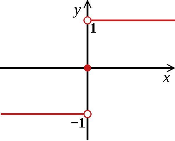
We cannot use our discrete examples above in this minimization algorithm, since the gradient descent would only work with continuous values. This is one of the limitations of the step function as an activation function. We tend to appy a softmax function instead.

Using a sigmoid activation will assign the value of a neuron to either 0 if the output is smaller than 0.5, or 1 if the neuron is larger than 0.5. The sigmoid function is defined by : \(f(x) = \frac {1} {1 + e^{-u}}\)

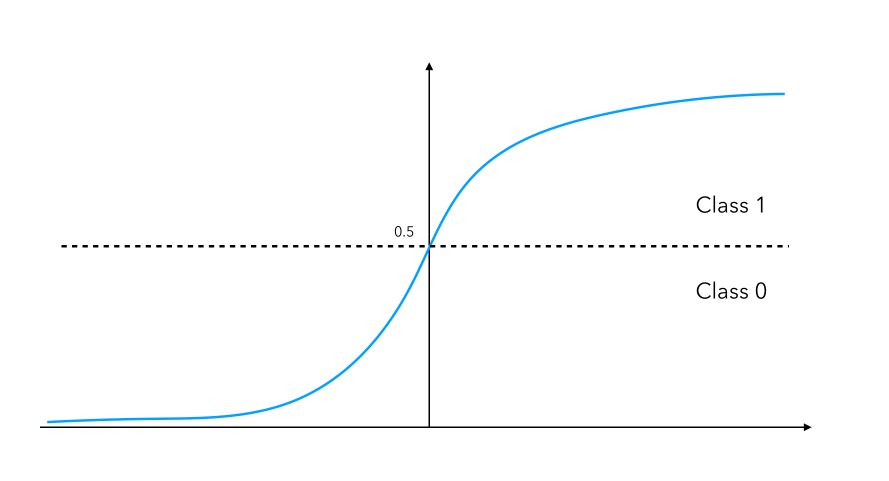
This activation function is smooth, differentiable (allows back-propagation) and continuous. We don’t have to output a 0 or a 1, but we can output probabilities to belong to a class instead. If you’re familiar with it, this version of the perceptron is a logistic regression with 0 hidden layers.

The perceptron can be seen as an error minimization algorithm. We choose the softmax function, a differentiable and continuous error function and try to minimize it by applying gradient descent.

We usually apply a log-loss error function. This error function applies a penalty to miscalssified points that is proportional to the distance of the boundary.

Multi-class

What if our problem involves more than 2 classes ? In such case, we apply a softmax function, that implies an exponential transformation to handle both positive and negative scores.

\[P(z_i \in C_i) = \frac {e^{z_i}} {\sum_j e^{j}}\]

The Python implementation of the sotfmax can be done in the following way :

def softmax(lst):
    exp_lst = np.exp(lst)
    sum_exp_lst = sum(exp_lst)

    result = []
    for i in exp_lst:
        result.append(float(i)/sum_exp_lst)

    return result

Cross-Entropy

We are now back to a 2 class scenario. Since we now have probabilities of having each point belonging to each class. What should we do based on that to select a model or another? We can compute the maximum likelihood, which is simply :

\(\prod_i p_i\) for each probability of a point belonging to a class it is assigned to.

However, working with products can be challenging and painful when we have a large amount of data. We prefer applying a negative log transformation. This is the cross-entropy.

A good model has a low cross-entropy, and a bad model has a high cross-entropy. One of the advantage of the cross-entropy is to be able to compute the individual error for each point, due to the summation property. Therefore, a misclassified point has a large individual error.

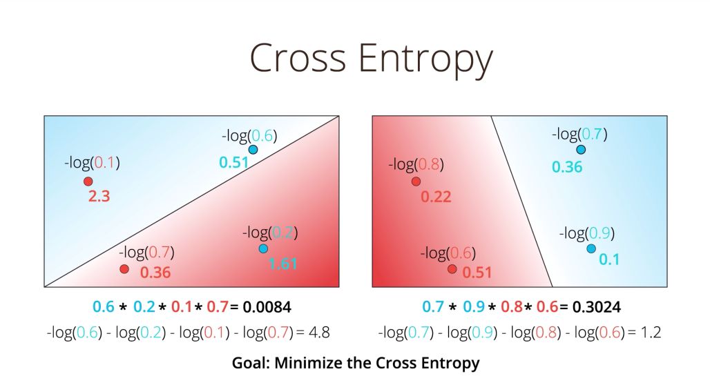
Our aim now becomes to minimize the cross-entropy !

The cross-entropy can be formalized as such :

\[CE = - \sum_i y_i \log{p_i} + (1-y_i) \log{1-p_i}\]

The cross-entropy can be computed in Python :

def cross_entropy(y, prob):
    return -1 * np.sum(y*np.log(prob) + (1-y)*np.log(1-prob))

As previously, we should consider applying the cross-entropy to multi-class cases :

\[CE = - \sum_j \sum_i y_{ij} \log{p_{ij}}\]

The main idea behind the variable \(y_{ij}\) is that we only add the probabilities of the events that occured. We can also take the average rather than the sum for the cross entropy by convention.

The ‘prob’ given above is actually known by the formula of the perceptron itself :

\[prob = \sigma (Wx_i + b)\]

Therefore, if we replace this value in the binary case :

\[CE = - \sum_i y_i \log{\sigma (Wx_i + b) } + (1-y_i) \log{1-\sigma (Wx_i + b)}\]

And in the multiclass framework :

\[CE = - \sum_j \sum_i y_{ij} \log{\sigma(Wx_{ij} + b)}\]

Error minimization

Our error function is now fully specified. The next step is to minimize this function through the iterations of the algorithm. We minimize this function by gradient descent. Our goal is to calculate the gradient of \(E\) at a point \(x = (x_1, \ldots, x_n)\) given by the partial derivatives

\[E = (\frac{\partial}{\partial w_1}E, \cdots, \frac{\partial}{\partial w_n}E)\]

There is a rather nice trick to apply here for the derivatives computation. Start by computing :

\[\frac{\partial}{\partial w_j} \hat{y} = \frac{\partial}{\partial w_j} \sigma (Wx + b)\] \[= (Wx + b)(1-(Wx + b)) \times \frac{\partial}{\partial w_j} (Wx + b)\] \[= \hat{y}(1-\hat{y}) \times \frac{\partial}{\partial w_j} (w_1 x_1 + \cdots + w_j x_j + \cdots + b)\] \[= \hat{y} (1-\hat{y}) x_j\]

This building block we be re-used when computing the two partial derivatives of the error function with respect to \(w_j\) and \(b_j\) :

\[\frac{\partial}{\partial w_j}E = \frac{\partial}{\partial w_j}(-y \log{\hat{y}} - (1-y) \log{1-\hat{y}})\] \[= -y \frac{\partial}{\partial w_j} \log{\hat{y}} - (1-y) \frac{\partial}{\partial w_j} \log{1-\hat{y}}\] \[= -y \frac{1}{\hat{y}} \frac{\partial}{\partial w_j} \hat{y} - (1-y) \frac{1}{1-\hat{y}} \frac{\partial}{\partial w_j} (1-\hat{y})\] \[= -y \frac{1}{\hat{y}} \frac{\partial}{\partial w_j} \hat{y} - (1-y) \frac{1}{1-\hat{y}} \frac{\partial}{\partial w_j} (1-\hat{y})\] \[= -y(1-\hat{y})x_j - (1-y)(\hat{y})x_j\] \[= -(y-\hat{y})x_j\]

Applying similar calculations, we can show that :

\[\frac{\partial}{\partial b}E = = -(y-\hat{y})\]

Overcall, the gradient can be seen in its vectorized form as :

\[∇E = -(y-\hat{y})(x_1, \cdots, x_n, 1)\]

We now have determined the gradients. For a “gradient descent”, we simply update the weights according to a learning rate in the inverse direction of the gradient :

\[w_j^{(i+1)} = w_j^{i} - \alpha (-(y-\hat{y})x_i)\]

Which can be rewritten as :

\[w_j^{(i+1)} = w_j^{i} + \alpha (y-\hat{y})x_i\]

And for the bias :

\[b^{(i+1)} = b^{i} + \alpha (y-\hat{y})\]

Where \(\alpha\) represents \(\frac{1}{m}\) of the original gradient since we moved in the average direction.

To summarize, the gradient descent algorithm is the following :

Initialize random weights : \(w_1, \cdots, w_n, b\)
For every point \(x_1, \cdots, x_n\) :
- For \(i \in 1 \cdots n\) :
  - Update \(w_j^* = w_j + \alpha (y-\hat{y})x_i\)
  - Update \(b^* = b + \alpha (y-\hat{y})\)
Repeat until the error gets smaller than a threshold

In the Perceptron algorithm, we split the weights update depending on the value of \(y - \hat{y}\) :

\(w_i = w_i + \alpha X_i\) if \(y - \hat{y}\) is positive
\(w_i = w_i - \alpha X_i\) if \(y - \hat{y}\) is negative

This is the exact same algorithm as the gradient descent !

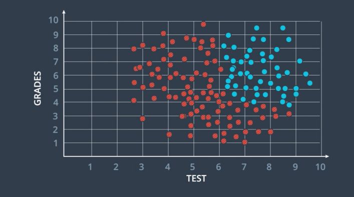
Building Neural Networks for Non-linear data

In most cases, the data is not linearly separable.

The basic idea is that we combine several linear models :

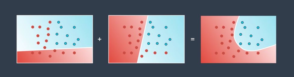
How do we combine those models ?

we have a probability for each point in the first model of belonging to the class blue class for example
we also have a probability for each point in the second model of belonging to the class blue
we add those probabilities
we map them in a sigmoid function
we get a probability in return

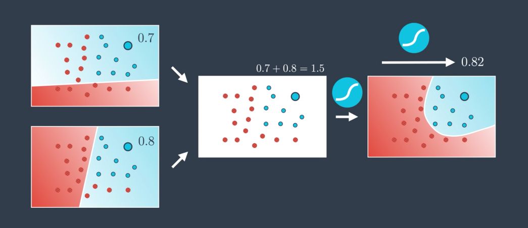
We can weight the models indiviually to assign more weight to a model than to another. Say that we want \(2/3\) of the overall weight on the first one. We simply apply a factor of 2 to the probabilites in the first model :

\[2 * 0.7 + 1 * 0.8\]

We can also add a bias to the individual models :

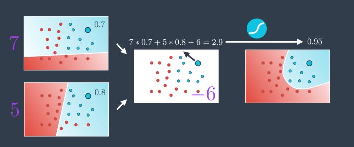
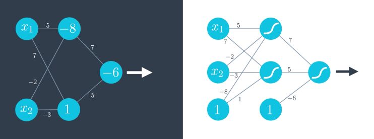
This is a new Perceptron ! This is the building block of Neural Networks. We take linear combinations of perceptrons to turn them into new perceptrons. We can visually represent this :

First we add a new perceptron as a linear combination of the 2 :

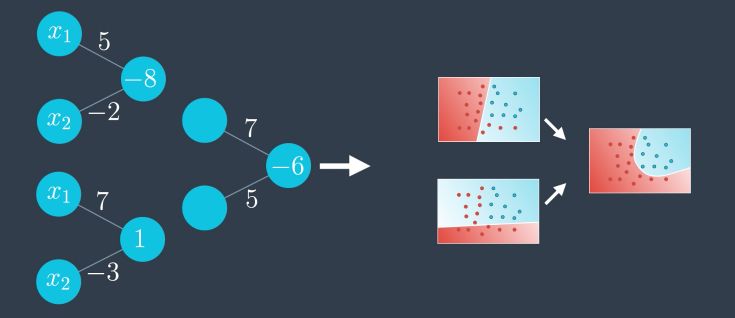
The outputs of the first 2 are the inputs of our perceptron :

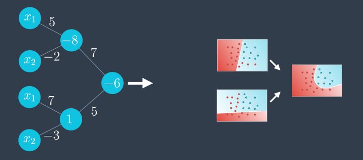
And since the first two perceptrons share the same inputs, we can group them :

As usual, we can represent the bias outside the neuron, and highlight the fact that we use the sigmoid activation function. This is how we systematically represent neural networks :

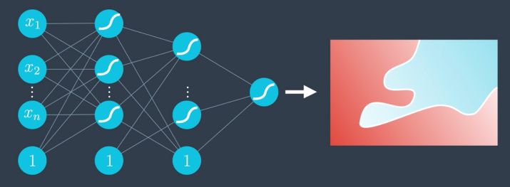
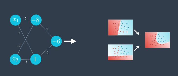
We can generalize this architecture even more into 3 categories :

an input layer
hidden layers
an output layer

All together, they form what is called : “Deep Neural Networks”.

The output layer can have as many neurons as we’d like, depending on the nature of the problem.

Full introduction to Neural Nets

Maël Fabien