
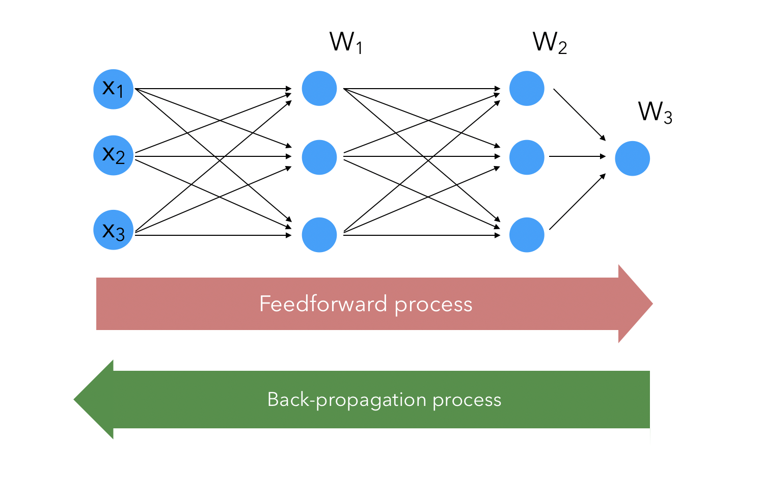
Let’s break down the maths behing Neural Networks. There are two main processes going on when a NN tries to learn a decision boundary :
- the feedforward process
- the back-propagation
They apply respectively to move forward with the weights we learned in order to compute the outcome, and to move backwards to update the weights once the outcome (an therefore the error) has been computed. You guessed it, the hard part is the back-propagation.
The Chain Rule
No spoil, but we’ll need to compute a big derivatives at some point in the learning process. How can we efficiently break down big derivatives into smaller steps ? Using the chain rule, yes. The chain rule can be applied here to drastically decrease the numbers of gradients to compute and the complexity of the calculus.
What the chain rule states is that when composing functions, the derivatives multiply :
\[\frac {\partial}{\partial t} f(x(t)) = \frac {\partial f} {\partial x} \frac {\partial x} {\partial t}\]And in more complex cases :
\[\frac {\partial}{\partial t} f(x(t), y(t)) = \frac {\partial f} {\partial x} \frac {\partial x} {\partial t} + \frac {\partial f} {\partial y} \frac {\partial y} {\partial t}\]Notation
“Notation in Deep Learning is important”, My Mom
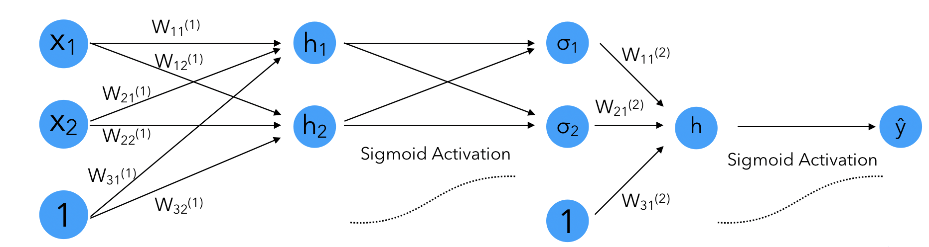
We wiil first cover the basic 1 Hidden Layer Neural Net case before extending to Deep Neural Nets. We’ll introduce basic notations :
- \(h = Wx + b\) is the outcome of an input that went through a neuron
- \(\hat{y} = \sigma(h)\) is \(h\) to which we applied an activation function
- \(E\) is the error. It could be the cross-entropy or the Mean Squared Error for example.
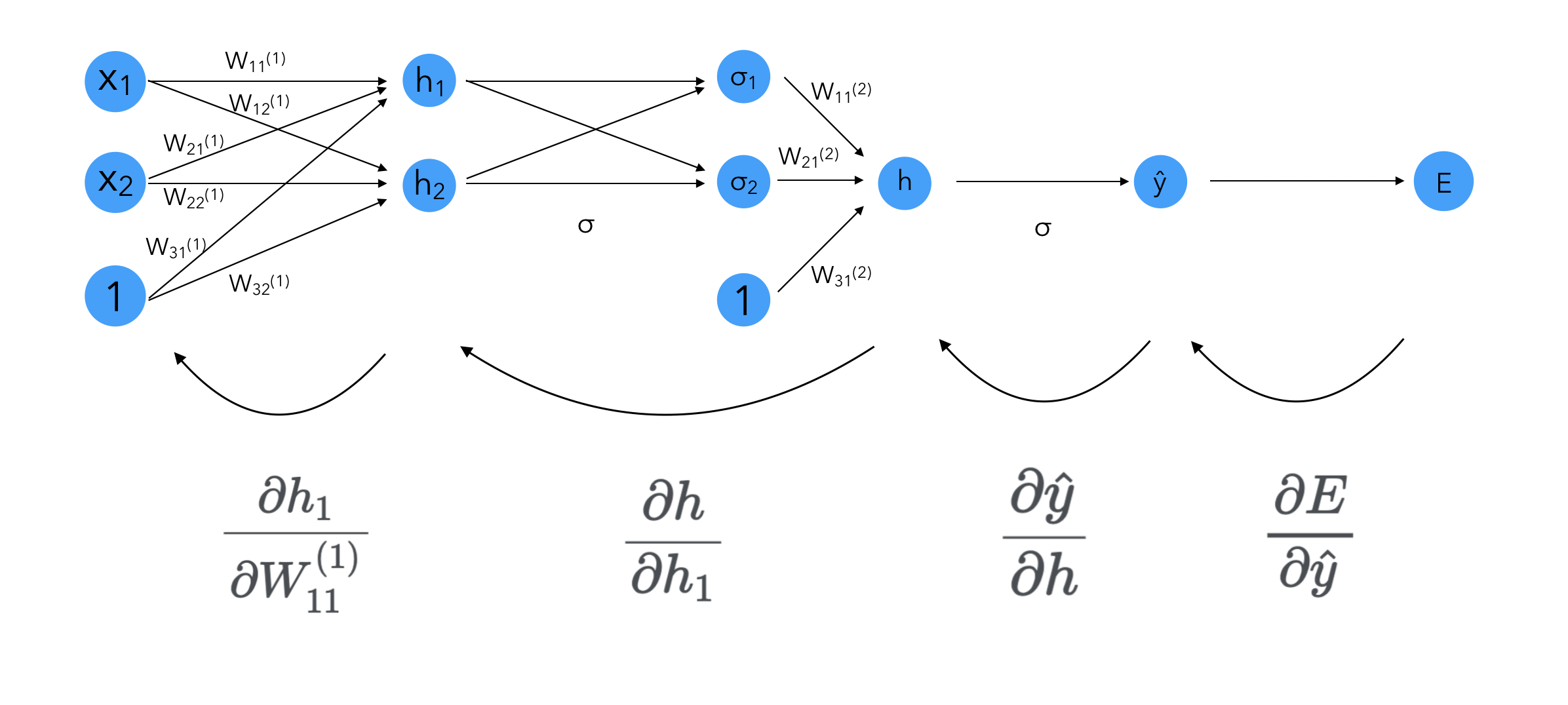
Let’s represent visually the Neuron Net we are talking about, and where the derivatives apply :
The derivatives apply in the back-propagation. In the back propagation, we compute : \(E = (\frac{\partial}{\partial W_{11}^{(1)}}E, \cdots, \frac{\partial}{\partial W_{31}^{(2)}}E)\)
We will see in the back-propagation section how to break down this problem.
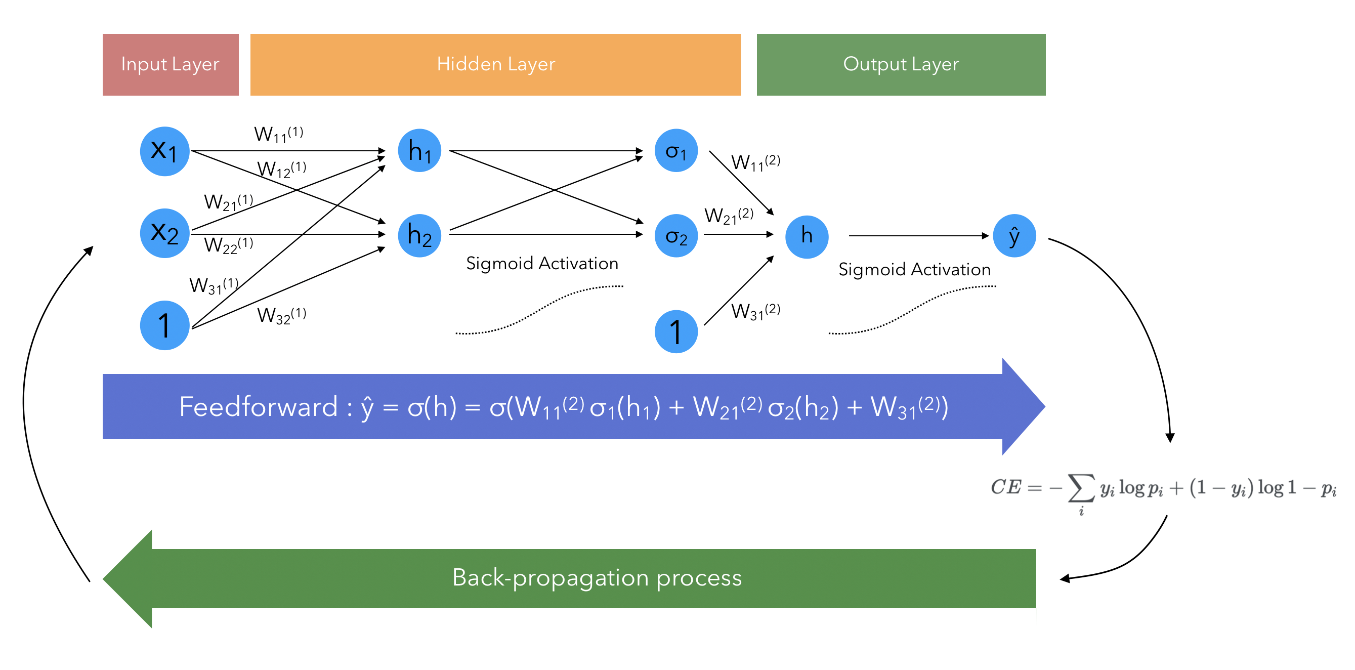
The Feedforward Process
The feedforward process is the process in Neural Networks that turns an input into an output. It describes the mathematical operations that allow to turn the input into an output. For example, on the example displayed above, with 2 hidden layers and 1 final layer :
\[\hat{y} = \sigma \circ W^{(2)} \sigma \circ W^{(1)} (x)\] \[\hat{y} = \sigma (h) = \sigma (W_{11}^{(2)} \sigma(h_1) + W_{21}^{(2)} \sigma(h_2) + W_{31}^{(2)}\]Where :
\[W^{(2)} = \begin{pmatrix} W_{11}^{(2)} & W_{12}^{(2)} \\ W_{21}^{(2)} & W_{22}^{(2)} \\ W_{31}^{(2)} & W_{32}^{(2)} \end{pmatrix}\] \[W^{(1)} = \begin{pmatrix} W_{11}^{(1)} & W_{12}^{(1)} & W_{13}^{(1)} \\ W_{21}^{(1)} & W_{22}^{(1)} & W_{23}^{(1)} \\ W_{31}^{(1)} & W_{32}^{(1)} & W_{33}^{(1)} \end{pmatrix}\]The error function will remain the same when computing how far out predicted output is from the true output :
\[CE(W) = - \frac{1}{m} \sum_i y_i \log{p_i} + (1-y_i) \log{1-p_i}\]The cost function is the sum of the losses of \(CE\) over all training examples \(m\) :
\[E = \frac{1}{m} \sum_m CE_m\]The Back-propagation
The second step of the process is to apply the Back-propagation. What this basically means is that we mapped our input to an output, and based on the performance of this mapping, we should be able to addjust the weights and bias in each layer accordingly.
We can compute the gradients with respect to each and every weight in the layers.
\[E = (\frac{\partial}{\partial W_{11}^{(1)}}E, \cdots, \frac{\partial}{\partial W_{31}^{(2)}}E)\]To update the gradient, we will do it individually :
\[W_{ij}^{(k)}* = W_{ij}^{(k)} - \alpha \frac{\partial E}{\partial W_{ij}^{(k)}}\]Feed-forwarding is nothing more than composing some functions. Therefore, back-propagation is nothing more than applying the chain rule to split the gradients into multiplicative derivatives.
We can compute the derivative of the error function as :
\[\nabla E = (\frac{\partial E}{\partial W_{11}^{(1)}}, \cdots, \frac{\partial E}{\partial W_{31}^{(2)}})\]Let’s break down the first derivative, since it’s the deepest dependency we have in our network so far :
Where \(h_i\) is the value taken by the output of a neuron at each step.
For example, in the first step :
\[h_1 = W_{11}^{(1)} x_1 + W_{21}^{(1)} x_2 + W_{31}^{(1)}\] \[h_2 = W_{12}^{(1)} x_1 + W_{22}^{(1)} x_2 + W_{32}^{(1)}\] \[h = W_{11}^{(2)} \sigma(h_1) + W_{21}^{(2)} \sigma(h_2) + W_{31}^{(2)}\]Notice how when computing the derivative with respect to one of the first weights of the network, you need the whole “chain” to be computed. And there is not only one way to reach neuron, since in deeper networks, we might go through other neurons. Therefore, by computing the partial derivatives, we will re-use them often.
We will need the derivative of the sigmoid function in the partial derivatives later on :
\[\sigma'(x) = \frac{\partial}{\partial x} \frac {1}{1+e^{-x}}\] \[= \frac{e^{-x}}{(1+e^{-x})^2} = \frac {1}{1+e^{-x}} \frac {e^{-x}}{1+e^{-x}} = \sigma(x) (1-\sigma(x))\]Using the expression of \(h\) we just defined, we can compute the partial derivatives ! For simplicity, we’ll use the mean squared error as an error metric : \(MSE(y, \hat{y}) = \frac{1}{2}(\hat{y}-y)^2\)
\[\frac{\partial E}{\partial \hat{y}} = \frac{\partial \frac{1}{2}(\hat{y}-y)^2 }{\partial \hat{y}} = \hat{y} - y\] \[\frac{\partial \hat{y}}{\partial h} = \sigma'(h) = \sigma(h) (1-\sigma(h))\]For the next derivative : \(\frac{\partial h }{\partial h_1}\), recall that \(h = W_{11}^{(2)} \sigma(h_1) + W_{21}^{(2)} \sigma(h_2) + W_{31}^{(2)}\). Therefore :
\[\frac{\partial h }{\partial h_1} = W_{11}^{(2)} \sigma'(h_1) = W_{11}^{(2)} \sigma(h_1) (1-\sigma(h_1))\]Finally, we need to compute \(\frac{\partial h_1 }{\partial W_{11}^{(1)}}\). Recall that \(h_1 = W_{11}^{(1)} x_1 + W_{21}^{(1)} x_2 + W_{31}^{(1)}\). Therefore :
\[\frac{\partial h_1 }{\partial W_{11}^{(1)}} = x_1\]We now have characterized all the steps of the learning process. For deeper neuronal nets, we’re just doing more of this steps, and making sure to re-use the gradients already computed accross layers.
Computing the partial derivatives is useless if we don’t update the weights using gradient descent :
\[W_{ij}^{(k)} = W_{ij}^{(k)} - \alpha \frac{\partial E}{\partial W_{ij}^{(k)}}\]Where \(\alpha\) is the learning rate. Progressively, we’ll be shifting in the right direction !
At this point, all that’s left is to re-apply the feedforward process with the updated weights, and so on, until you reach your maximum number of iterations or any other stopping criteria.