
When building your Deep Learning model, activation functions are an important choice to make. In this article, we’ll review the main activation functions, their implementations in Python, and advantages/disadvantages of each.
Linear Activation
Linear activation is the simplest form of activation. In that case, \(f(x)\) is just the identity. If you use a linear activation function the wrong way, your whole Neural Network ends up being a regression :
\[\hat{y} = \sigma(h) = h = W^{(2)} h_1 = W^{(1)} W^{(2)} X = W' X\]Linear activations are only needed when you’re considering a regression problem, as a last layer. The whole idea behind the other activation functions is to create non-linearity, to be able to model highly non-linear data that cannot be solved by a simple regression !
ReLU
ReLU stands for Rectified Linear Unit. It is a widely used activation function. The formula is simply the maximum between \(x\) and 0 :
\[f(x) = max(x, 0)\]To implement this in Python, you might simply use :
def relu(x) :
    return max(x, 0)
The derivative of the ReLU is :
- \(1\) if \(x\) is greater than 0
- \(0\) if \(x\) is smaller or equal to 0
def der_relu(x):
    if x <= 0 :
        return 0
    if x > 0 :
        return 1
Let’s simulate some data and plot them to illustrate this activation function :
import numpy as np
import matplotlib.pyplot as plt

# Data which will go through activations
x = np.linspace(-10,10,100)

plt.figure(figsize=(12,8))
plt.plot(x, list(map(lambda x: relu(x),x)), label="relu")
plt.plot(x, list(map(lambda x: der_relu(x),x)), label="derivative")
plt.title("ReLU")
plt.legend()
plt.show()
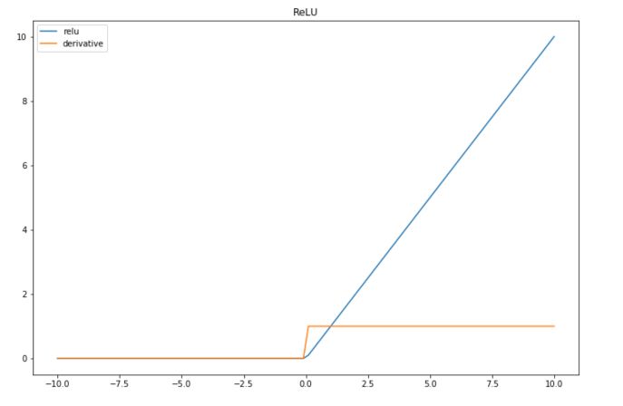
| Advantage | Easy to implement and quick to compute |
| Disadvantage | Problematic when we have lots of negative values, since the outcome is always 0 and leads to the death of the neuron |
Leaky-ReLU
Leaky-ReLU is an improvement of the main default of the ReLU, in the sense that it can handle the negative values pretty well, but still brings non-linearity.
\[f(x) = max(0.01x, x)\]The derivative is also simple to compute :
- \(1\) if \(x>0\)
- \(0.01\) else
def leaky_relu(x):
    return max(0.01*x,x)

def der_leaky_relu(x):
    if x < 0 :
        return 0.01
    if x >= 0 :
        return 1
And we can plot the result of this activation function :
plt.figure(figsize=(12,8))
plt.plot(x, list(map(lambda x: leaky_relu(x),x)), label="leaky-relu")
plt.plot(x, list(map(lambda x: der_leaky_relu(x),x)), label="derivative")
plt.title("Leaky-ReLU")
plt.legend()
plt.show()
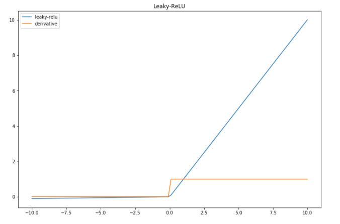
| Advantage | Leaky-ReLU overcomes the problem of the death of the neuron linked to a zero-slope. |
| Disadvantage | The factor 0.01 is arbitraty, and can be tuned (PReLU for parametric ReLU) |
ELU
Exponential Linear Units (ELU) try to make the mean activations closer to zero, which speeds up learning.
\(f(x) = x\) if \(x>0\), and \(a(e^x -1)\) otherwise, where \(a\) is a positive constant.
The derivative is :
- \(1\) if \(x > 0\)
- \(a * e^x\) otherwise
If we set \(a\) to 1 :
def elu(x):
    if x > 0 :
        return x
    else :
        return (np.exp(x)-1)

def der_elu(x):
    if x > 0 :
        return 1
    else :
        return np.exp(x)
plt.figure(figsize=(12,8))
plt.plot(x, list(map(lambda x: elu(x),x)), label="elu")
plt.plot(x, list(map(lambda x: der_elu(x),x)), label="derivative")
plt.title("ELU")
plt.legend()
plt.show()
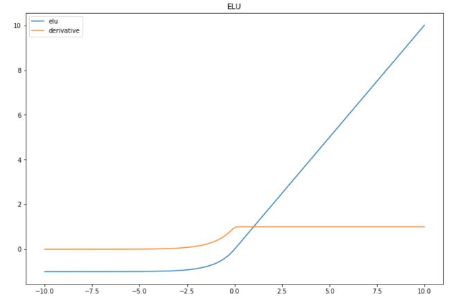
| Advantage | Can achieve higher accuracy than ReLU |
| Disadvantage | Same as ReLU, and a needs to be tuned |
Softplus
The Softplus function is a continuous approximation of ReLU. It is given by :
\[f(x) = log(1+e^x)\]The derivative of the softplus function is :
\[f'(x) = \frac{1}{1+e^x}e^x\]You can implement them in Python :
def softplus(x):
    return np.log(1+np.exp(x))

def der_softplus(x):
    return 1/(1+np.exp(x))*np.exp(x)
plt.figure(figsize=(12,8))
plt.plot(x, list(map(lambda x: softplus(x),x)), label="softplus")
plt.plot(x, list(map(lambda x: der_softplus(x),x)), label="derivative")
plt.title("Softplus")
plt.legend()
plt.show()
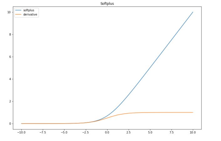
| Advantage | Softplus is continuous and might have good properties in terms of derivability. It is interesting to use it when the values are between 0 and 1. |
| Disadvantage | As ReLU, problematic when we have lots of negative values, since the outcome gets really close to 0 and might lead to the death of the neuron |
Sigmoid
Sigmoid is one of the most common activation functions in litterature these days. The sigmoid function has the following form :
\[f(x) = \frac{1}{1+e^{-x}}\]The derivative of the sigmoid is :
\[f'(x) = - e^{-x} \frac{1}{(1+e^{-x})^2} = \frac {1 + e^{-x} -1}{(1+e^{-x})^2}\] \[= \frac {1}{1+e^{-x}} (1-\frac {1}{1+e^{-x}}) = f(x)(1-f(x))\]In Python :
def softmax(x):
    return 1/(1+np.exp(-x))

def der_softmax(x):
    return 1/(1+np.exp(-x)) * (1-1/(1+np.exp(-x)))
plt.figure(figsize=(12,8))
plt.plot(x, list(map(lambda x: softmax(x),x)), label="softmax")
plt.plot(x, list(map(lambda x: der_softmax(x),x)), label="derivative")
plt.title("Softmax")
plt.legend()
plt.show()
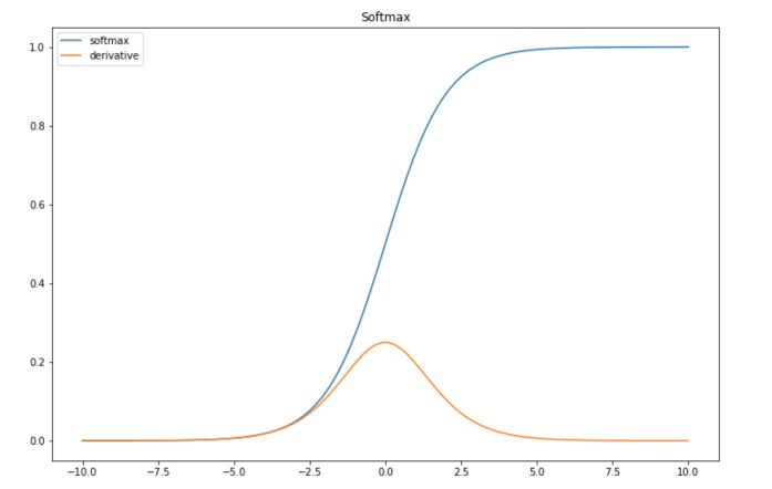
It might not be obvious when considering data between \(-10\) and \(10\) only, but the sigmoid is subject to the vanishing gradient problem. This means that the gradient will tend to vanish as \(x\) takes large values.
Since the gradient is the sigmoid times 1 minus the sigmoid, the gradient can be efficiently computed. If we keep track of the sigmoids, we can compute the gradient really quickly.
| Advantage | Interpretability of the output mapped between 0 and 1, compute gradient quickly |
| Disadvantage | Vanishing Gradient |
Hyperbolic Tangent
Hyperbolic tangent is quite similar to the sigmoid function, expect is maps the input between -1 and 1.
\[f(x) = tanh(x) = \frac {sinh(x)}{cosh(x)} = \frac {e^x - e^{-x}}{e^x + e^{-x}}\]The derivative is computed in the following way :
\[f'(x) = \frac{\partial}{\partial x} \frac{sinh(x)}{cosh(x)}\] \[= \frac { \frac{\partial}{\partial x} sinh(x) cosh(x) - \frac{\partial}{\partial x} cosh(x) sinh(x) } {cosh^2(x)}\] \[= \frac { cosh^2(x) - sinh^2(x) } {cosh^2(x)}\] \[= 1 - \frac { sinh^2(x) } { cosh^2(x) }\] \[= 1 - tanh^2(x)\]Implement this in Python :
def hyperb(x):
    return (np.exp(x)-np.exp(-x)) / (np.exp(x) + np.exp(-x))

def der_hyperb(x):
    return 1 - ((np.exp(x)-np.exp(-x)) / (np.exp(x) + np.exp(-x)))**2
And plot it :
plt.figure(figsize=(12,8))
plt.plot(x, list(map(lambda x: hyperb(x),x)), label="hyperbolic")
plt.plot(x, list(map(lambda x: der_hyperb(x),x)), label="derivative")
plt.title("Hyperbolic")
plt.legend()
plt.show()
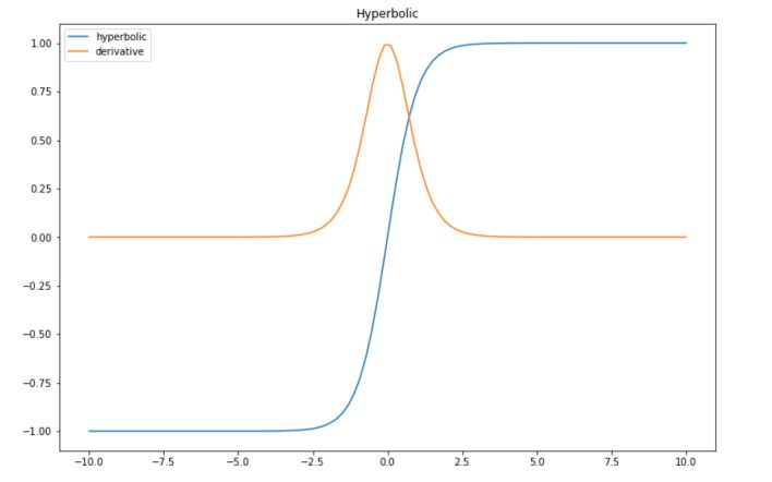
| Advantage | Efficient since it has mean 0 in the middle layers between -1 and 1 |
| Disadvantage | Vanishing gradient too |
Arctan
This activation function maps the input values in the range \((− \pi / 2, \pi / 2)\). It is the inverse of a hyperbolic tangent function.
\[f(x) = arctan(x)\]And the derivative :
\[f'(x) = \frac {1} {1+x^2}\]In Python :
def arctan(x):
    return np.arctan(x)

def der_arctan(x):
    return 1 / (1+x**2)
And plot it :
plt.figure(figsize=(12,8))
plt.plot(x, list(map(lambda x: arctan(x),x)), label="arctan")
plt.plot(x, list(map(lambda x: der_arctan(x),x)), label="derivative")
plt.title("Arctan")
plt.legend()
plt.show()
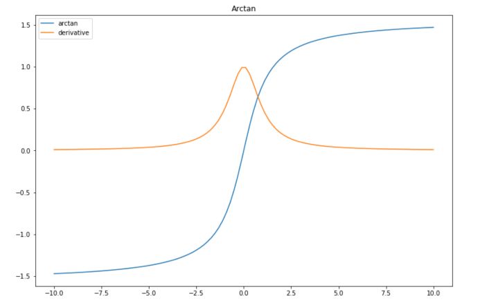
| Advantage | Simple derivative |
| Disadvantage | Vanishing gradient |